Abstract
Typical berm erosion and accretion are closely related to the beach-face slope. Empirical equation for prediction of the beach-face slope is proposed. The beach-face slope is expressed as a function of the wave period and the bed sediment grain size. Coefficients in the equation are obtained from three sets of carefully chosen laboratory data through a multiple linear regression with two independent variables using SPSS version 22. The computed correlation coefficient is as high as 0.983, which is believed to justify the validity of the present formulation. A shore profile is split into beach-face and underwater bed profile in the surf zone, and described with two straight lines. Possibility of using the beach-face slope strategically for warning of future berm erosion at the site is proposed.
1. Introduction
On-offshore or cross-shore sediment transport problem is a very complex problem which involves wave breaking, tidal variation, and offshore bar formation and movement. Beach-face is a special place where water is dynamically mixed with air bubbles, waves run up and down, and bed sediment transports affected by infiltration, exfiltration and groundwater level. Interestingly the beach-face exhibits fairly straight shape or constant slope compared to underwater surf zone with wavy geometry.
The shore zone has been heavily treated as a defense line. Especially it protects land from disasters like storm, storm surge or tsunami. Worldwide efforts are undergoing to preserve shore capacity to prevent natural disasters at many coastal sites. Special structures have been designed and constructed for the purpose, and beach nourishment has also been frequently used to preserve beach width. For example, Haeundae beach, Busan, Korea has recently suffered serious erosion, been nourished with sand to some extent, and still urgent optimum countermeasures are needed to control the erosion at the site.
The sediment transport around shoreline is induced by many physical parameters, e.g. winds, waves, and long-shore currents. Underwater sediment transport mechanism has often been studied in separate categories like wave, current, wave and current-driven sediment transport. Although understanding of sediment transport in wave current environment has significantly progressed up to the present, many areas still need further research works, e.g. mud-sand mixture problem, bed-form prediction, and cross-shore sediment transport and profile change. The effect of grain size and sorting on coastal sediment transport has not yet been intensively studied, either. Armouring is another important factor affecting scour around coastal or ocean structures.
The sediment transport around shoreline has often been described by combination of two different modes; the longshore sediment transport (O’Connor et al., [1]) and the cross-shore sediment transport. We will look into the cross-shore sediment transport in this paper.
The cross-shore sediment transport has been studied by many researchers since decades ago because of its relationship with shore protection. The cross-shore sediment transport is affected by several factors, i.e. wave height, wave period, wave power, skewness or asymmetry of water level, particle velocity, or acceleration during wave period, dispersion due to wave breaking, undertow current, bed material properties, balance between bed load and suspended load, and local bed slope. Individual researchers argue different relative importance between the above factors. Onshore or offshore boundary conditions also affect the shore profile changes. Watanabe et al. [2], Kajima et al. [3], Bailard [4], respectively, proposed theories or numerical models for cross-shore sediment transport. Bruun [5] proposed equilibrium profile concept which is an output of cross-shore sediment transport description. The equilibrium profile represents a state that no net cross-shore sediment flux occurs along the profile for a given steady wave condition. Donnelly et al. [6] studied the cross-shore sediment transport over barrier islands. The sediment transport and profiles at barrier islands are distinguished from other types of onshore profiles because of overwash over the barriers. Aagaard et al. [7] looked at detailed temporal and spatial behavior of suspended sediment in the surf zone in their numerical modeling work of sediment transport, instead of using empirical formulae for bed load or total load. Some researchers presented comparison results of existing cross-shore models, e.g. Abreu et al. [8] compared a few cross-shore sediment transport models, and recommended further improvement of models. Two-dimensional wave flume is an adequate device to study the cross-shore sediment transport, because it is not interfered by long-shore current or long-shore sediment transport, the condition of which hardly exists at real fields. More elaborate laboratory experiments have also been carried out, e.g. Dubarbier et al. [9] used light weight sediment for their experimental and numerical modelling work on cross-shore sediment transport.
Some researchers tried to quantify the effect of the wave skewness or particle velocity asymmetry on the cross-shore sediment transport (Doering and Bowen [10], Rakha and Deigaard [11], Doering et al. [12], Sancho et al. [13], Rocha et al. [14], Grasso [15]). Baldock et al. [16] argued that the effect of long waves on the shore bed profile is non-negligible.
Average bed slope within a range of horizontal distance has been studied for various purposes. Explicit forms of equations for the average bed slope within the surf zone or the bed slope at a specific location along offshore distance were proposed by a few researchers, and equations for the beach-face slope were also proposed by other researchers.
Hanson and Kraus [17] made use of Dean’s [18] equation with a power function for the equilibrium bed profile shape, and deduced an equation for the average bed slope within the surf zone from integration of the equilibrium bed profile equation. They used it in their program GENESIS. They assigned the offshore limit as the location, the offshore side of which cross-shore sediment transport does not occur. Equations of the model read:
where is the local water depth, is a scale parameter known as a function of the median grain size, is the offshore distance from an origin, is the angle between the local bed surface and the horizon, is the local bed slope, is the maximum water depth of long-shore sediment transport, is the deep water wave height, and is the deep water wave length. For example, they suggested as for 0.4 mm, and for 0.4 10 mm, respectively. However, the above approach is limited to very small deep water wave height condition in Eq. (3) describing the maximum water depth of long-shore sediment transport, which can produce negative water depth for large deep water wave height. Another problem of the above approach is that Dean’s equilibrium profile equation is not applicable at the origin of axis () because of singularity, which is not valid for description of the slope near beach-face.
Larson and Kraus [19] adopted an empirical equation for the bed slope seaward the wave break point while developing their cross-shore sediment transport model, SBEACH, that is:
where, is the breaker ratio (), and is the similarity parameter. However, the equation for the local bed slope seaward of the break point is different from much steeper beach-face slope.
Sunamura and Horikawa [20] proposed an index to distinguish net sediment transport direction whether it is in the onshore or offshore direction, that is:
where is the index coefficient, is the initial uniform bed slope in the surf zone, and is the median grain size. could be regarded as a scale parameter of the above equation. Sunamura and Horikawa suggested that if is larger than 8, the sediment transport direction is offshore; if is smaller than 4, the sediment transport direction is onshore; and if is between 4 and 8, the sediment transport direction is neutral. Taking a central value of 6 for as the neutral sediment transport direction, the above equation can be rearranged into the following form:
The above equation could be regarded as the equilibrium slope for given wave and bed material conditions. However, the bed slope in the above equation is thought to be the mean slope from the beach to the point of the offshore limit water depth of sediment transport. Thus, it is not possible to use the above equation for prediction of the beach-face slope.
Walgreen et al. [23] studied the effect of grain size sorting on the formation of sand ridges with analysis of field data. Hoque and Asano [21] developed a numerical model coupling wave motion and groundwater flow over a uniform slope. They emphasized the importance of the effect of infiltration and exfiltration on sediment transport. Kelly and Dodd [22] developed a numerical model to investigate swash on erodible beaches, and emphasized the importance of coupling of water and bed motions, worked on the bed evolution and the maximum wave run-up.
The bed slope at the beach-face may be steepest along cross-shore bed profile. The bed slope generally gets milder as the water gets deeper with exception around offshore bars. Let’s define the beach-face slope as a representative slope of the beach-face, and more specifically the slope of the beach-face on the mean sea level. The beach-face slope is relatively easy to measure compared to submerged zone slope. The beach-face is also called as swash zone, or foreshore depending on viewer’s viewpoint. It could be defined as the place where waves run up and backrush.
Previous research results on the beach-face slope include Sunamura [24], Anthony [25], Masselink and Li [26], and Reis and Gama [27].
Sunamura [24] proposed empirical formulae for prediction of the beach-face slope. He derived a non-dimensional parameter, first, where is the breaking wave height, is the acceleration due to gravity, is the median grain size of the bed material, and is the wave period, and fitted curves onto some laboratory data and field data, respectively. Sunamura’s equations are:
Although Sunamura’ predictions show similar trend with the data he used, comparison figures of data and prediction curves display wide scattering. Perhaps the above non-dimensional parameter he chose may not be enough to reflect the inherent detailed physics. The beach-face slope increases with the wave period in his formulas, the trend of which disagrees with some existing data (Wise et al. [28]).
Anthony [25] suggested that beach parameters like the Iribarren number which includes the bed slope are better indicators of beach morphodynamic type, such as reflective or dissipative, than sediment size. However, Anthony’s results are not in a form to predict the beach-face slope.
Masselink and Li [26] proposed a numerical model incorporating micro-processes to describe the relationship between the beach-face slope and infiltration, exfiltration and groundwater level. They concluded that sand beaches are not much affected by the infiltration or exfiltration in contrast to gravel beaches.
Reis and Gama [27] induced a relationship between the sand size, offshore wave height, and the beach-face slope by introducing the so-called “constructal law” (Bejan, [29]). They obtained the beach-face slopes by adjusting a straight line around mean sea level. Although they did not show an explicit form of empirical prediction equation, their argument can be expressed in the following form:
where is the scaling coefficient decided by field conditions including the grain sphericity, porosity, and the fluid viscosity. The above relationship was examined to a group of field data. However, the data they used are confined in relatively small offshore wave heights. They plotted field data onto their theoretical group of curves, and didn’t mention the agreement level between the two.
As regards methodology to predict the beach-face slope, Sunamura’s and Reis and Gama’s equations are available, but their equations incorporate weak points. Further refinement of the previous formulae is tried in this paper.
2. Determination of empirical functional form for beach-face slope
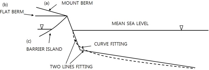
Field sea bed profile shapes cannot be standardized due to diverse site-specific parameters, e.g. external forces and bed material properties. Although there is no standard berm pattern above beach-face, we can think of some typical berm types, i.e. mount berms, flat berms, or island berms. Each type means (a) bed level becomes higher further inland, (b) bed level stays more or less flat, (c) bed level becomes lower after a island summit, and meets another mean sea level, respectively, see Fig. 1. The onshore berm pattern affects onshore boundary condition for bed profile changes. When condition (c) is applied, i.e. almost parallel two shorelines run along a barrier island, overwash takes an important role for shoreline movement. The pattern of shoreline movement of barrier islands is distinguished from that of landside beaches.
Equilibrium profile is a useful concept. If a profile is in equilibrium, no net sediment transport occurs at all points of a beach profile, and the profile does not change in time. However, in reality shore profiles always change, and equilibrium status is not reached at all. Nevertheless the equilibrium profile concept may be useful for engineering purpose. If we know that any profile is close to the equilibrium one, sediment transport and the bathymetric status at the site could be considered as almost steady.
Dean’s equilibrium bed profile equation is relatively simple, and has been referred by many people. Dean’s equilibrium equation is of a power form; the onshore-side boundary slope is large, and the bed slope becomes milder with the offshore distance from the shoreline, the trend of which is generally correct at fields, if offshore bars are ignored. However, the slope towards the onshore boundary becomes unlimited as the offshore distance approaches zero, and the offshore limit the equation can be applied has not well been defined.
Fig. 1Berm types over beaches
The beach-face slope is generally steeper than other part of the bed profile, or the average bed slope in the surf zone. The beach-face profile is more or less straight within the beach-face width. For example, the beach-face slopes at Profile Line 188, Duck, NC, USA of Birkmeier [30] during several months look straight, and the crest points of the profiles have not moved much, which means the berm has not suffered serious erosion or accretion during the period, while the surf zone suffered serious morphological changes, see Fig. 2. Even though the above site is just an example, it demonstrates typical behavior of the bed profile change. In contrast to the beach-face the main bed morphology in the surf zone experienced wild changes, especially during storm season, and one or multiple sand bars developed within the surf zone at the above example shore, see Fig. 3. The sand bars are not necessarily straight in plane, or parallel with the shoreline. They behave like sand dunes, migrates onshore-ward or offshore-ward depending on the variation of wave climate. A detailed field bathymetric survey on an east coast of Korea has shown that each bar is circular in plane rather than straight, and moves around with a high speed (Lee, [31]).
Thus, two straight lines could be used to describe the whole shore bed profile between the beach-face to the offshore limit for sediment transport. The straight line representing the bed level in the surf zone is not an accurate profile, but it is a kind of filtered or spatial moving-averaged bed profile getting rid of wavy components like offshore bars. We first describe the beach-face slope.
Fig. 2Example of bed profile changes at Profile Line 188 (after Birkmeier [30])
![Example of bed profile changes at Profile Line 188 (after Birkmeier [30])](https://static-01.extrica.com/articles/14904/14904-img2.jpg)
The beach slope is related to many physical parameters, e.g. tidal range, wave parameters including wave height, wave period, wave direction, wave duration, and bed material parameters including median grain size, local grain size distribution, grain size variation along profile, and berm pattern.
Fig. 3Example morphology showing moving offshore bars in surf zone at Profile Line 188 (after Birkmeier [30])
![Example morphology showing moving offshore bars in surf zone at Profile Line 188 (after Birkmeier [30])](https://static-01.extrica.com/articles/14904/14904-img3.jpg)
It may not be easy to develop a general prediction equation of the beach-face slope applicable to any coastal sites. We consider some simplified situations only:
- Zero tidal range is assumed.
- Flat onshore berms are considered.
- The beach slope is assumed to be in equilibrium.
- Wave direction is assumed to be normal to the shoreline.
- Medium grain size is uniform along the bed profile.
We first try to identify the most important variables which affect the beach-face slope.
First, waves are important external force to affect the beach morphology. Field waves are not only multi-frequency, but also multi-directional random waves. However, laboratory data from two-dimensional wave flumes can be considered as better controlled data. Furthermore, data for regular waves can represent the effect of the wave period or wave height more clearly and explicitly. Therefore, as the first step it would be meaningful to draw out an empirical formula for the beach slope as a function of regular wave parameters by using laboratory regular wave data rather than using field multi-directional random wave data or laboratory long-crested random wave data.
The effect of the offshore wave height on the equilibrium profile must be significant. For example, the offshore wave height determines the breaking water depth, and the offshore critical water depth for sediment transport. The surf zone width, the undertow strength, and the turbulence-induced dissipation strongly depends on the deep water wave height. However, it has been known that the local wave height is closely dependent on the local water depth, i.e. the local wave height does not have strong link with the offshore wave height for spilling breakers:
The wave breaker ratio is known to be weakly dependent to the wave steepness and the local bed slope. Ignoring wave-induced setup, treating as constant for spilling breakers, the wave height near the shoreline becomes identical regardless of the deep water wave height, see Fig. 4. The wave-induced set-up may not be ignorable for high waves, but the order of magnitude is relatively small compared to the wave height itself, and the shoreline retreat due to the wave set-up is expected not to be large. The beach-face slope may not be much influenced by the wave set-up, or the resultant shoreline movement because of its almost uniform attribute within the beach-face range. Therefore, we decide not to include the wave height as an independent variable to the dependent variable, beach-face slope. Watanabe et al. [2] showed their laboratory experimental results for the same wave period and different wave heights, and the results demonstrate the wave height affects the width of bed profile change rather than the beach-face slope, see Fig. 5.
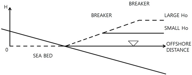
Fig. 4. Wave height distribution for spilling breaker type
Fig. 5Example of small dependency of beach-face slope on wave height (after Watanabe [2])
![Example of small dependency of beach-face slope on wave height (after Watanabe [2])](https://static-01.extrica.com/articles/14904/14904-img5.jpg)
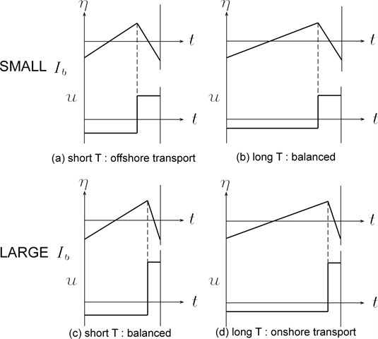
As an important parameter of sea waves, the wave period strongly affects bed morphology through fluid motion characteristics, e.g. the wave skewness, or water particle velocity asymmetry, see Fig. 6. Both the bed slope and the wave period are strongly related to the wave skewness. The equilibrium beach-face slope is inferred to be dependent on the wave period here.
Next, the bed material properties are important parameters affecting the beach-face slope. There are many parameters to describe non-cohesive sediment properties, e.g. the median grain diameter, variance, and skewness. The median diameter may be the most important parameter between them.
Thus, we propose an empirical formula for the equilibrium beach-face slope as a function of the wave period, and the bed medium grain size as:
where is the beach-face slope (), and is the angle between the beach-face slope and the horizon. The above equation can be regarded as a function of the deep water wave length and the median grain size, too. Introducing power relationships between the beach-face slope and the two independent variables, the wave period, and the median grain diameter:
Fig. 6Schematic diagram of relation between bed slope, wave period, and net sediment transport direction
In order to find three coefficients in the above equation either rational reasoning or a statistical analysis of data is needed. Available existing data sets are as follows:
a) Watanabe et al. [2]
Watanabe et al. carried out laboratory experiments on cross-shore sediment transport at a medium-sized wave flume. They started experiments on uniform-sloped sand bed, and presented final equilibrium profiles for many cases combining several wave conditions, bed sand grain sizes, and initial bed slopes. Although they did not explicitly shown the beach-face slope data, the slopes can be read from their profile figures. Uniform initial bed slopes were used for their experiment.
Table 1Watanabe et al.’s experimental cases (initial bed slope = 0.1) [2]
Case | Deep water wave height (m) | Wave period (s) | Grain size (mm) | Beach-face slope |
A-122 | 0.058 | 1.5 | 0.2 | 0.231 |
A-132 | 0.054 | 2.0 | 0.2 | 0.211 |
B-123 | 0.077 | 1.5 | 0.7 | 0.263 |
B-134 | 0.082 | 2.0 | 0.7 | 0.240 |
b) Kajima et al. [3]
Kajima et al. carried out laboratory experiments at a large wave flume, and presented time-varying profiles for many cases: changing wave conditions, bed grain size, and initial bed slope. Uniform initial bed slopes were used for their experiment.
Table 2Kajima et al.’s experimental cases [3]
Case | Wave height (m) | Wave period (s) | Grain size (mm) | Initial bed slope | Beach-face slope |
2-1 | 1.76 | 6.0 | 0.47 | 0.03 | 0.140 |
2-2 | 0.73 | 9.0 | 0.47 | 0.03 | 0.130 |
3-1 | 1.07 | 9.1 | 0.27 | 0.05 | 0.110 |
3-2 | 1.05 | 6.0 | 0.27 | 0.05 | 0.130 |
c) Wise et al. [28]
Wise et al. carried out experiments at a large wave flume Supertank for cases of various conditions, and used the data for validation of their cross-shore sediment transport numerical model. They started each experiment from non-uniform-sloped bed profiles, and obtained modified bed profiles after some time. They confined the wave periods within a narrow range for their experiments, and used one bed material only. Their experimental cases include many random wave cases, and five regular wave cases. Four of their regular wave experimental results are select for our statistical analysis here to distinguish the effect of the wave period, while one case for overwashing with regular waves is not included in our statistical analysis.
Table 3Wise et al.’s large water tank experiments for regular waves [28]
Case | Wave height (m) | Wave period (s) | Grain size (mm) | Beach-face slope | Remarks |
P1E2 | 0.8 | 4.5 | 0.22 | 0.140 | Eroded beach |
PGA | 0.8 | 3.0 | 0.22 | 0.170 | Eroded beach |
PJC | 0.7 | 3.0 | 0.22 | 0.160 | With narrow-crested mound |
PKC | 0.7 | 3.0 | 0.22 | 0.150 | With broad-crested mound |
The above three sets of data were used to find the three coefficients in Eq. (15). The prediction equation was first transformed into a linear equation by taking logarithm on both sides. Then the linear regression module with multiple independent variables in SPSS-version 22 was used for the regression analysis (Levesque, [32]). Analysis results show high correlation coefficient () of 0.983. The three coefficients in the prediction equation, , , , are 0.332, –0.416, 0.122, respectively, see Table 4.
Table 4Results of regression analysis of three sets of data
Variables | Non-standardized coefficients | Standardized coefficient | Significance level | |
Standard error | ||||
–1.103 | 0.0412 | 0.000 | ||
–0.416 | 0.020 | –0.968 | 0.000 | |
0.122 | 0.030 | 0.185 | 0.010 | |
Eq. (15) is rewritten with coefficients found:
where is the wave period (s), and is the median grain size (mm). The above new empirical equation expresses the trends that the longer the wave period, the milder the beach-face slope; the coarser the median grain size, the steeper the slope.
Now we apply the above new empirical equation, Sunamura’s equation, and Reis and Gama’s equation to the previous three data sets for inter-comparison with laboratory data, see Table 5. While using Eq. (11) of Weis and Gama, the coefficient was differently chosen to produce best agreement with laboratory measurements for each set of data.
Table 5 shows that the mean absolute error of the present equation, Eq. (16), is 4 times smaller than Sunamura’s equation, and 9 times smaller than Reis and Gama’s equation. It should be noted that the data used for inter-comparison was used for extracting Eq. (16). Nevertheless, it is believed that the beach-slope is strongly affected by both the wave period, and the bed grain size, and less influenced by the wave steepness (wave height over wave length), or the wave height, which are included in Sunamura’s equation, and Reis and Gama’s equation, respectively.
It is noted that the data used for the above regression are within limited ranges, i.e. from 1.5 to 9 seconds of the wave period, and from 0.2 to 0.7 mm of the median grain size. It would be acceptable to predict a beach-face slope for conditions within the ranges by using the above new equation, but using the above equation for extrapolation cases should be careful, until it is valicated to conditions of wider ranges, or additional regression work is done with additional data of wider ranges.
Table 5Comparison of empirical equations, Sunamura [24], Reis and Gama [27], and Eq. (16) and three sets of laboratory beach-face slope measurements
Case number | Lab. data | Sunamura | Reis and Gama | New (Eq. (16)) | |
Watanabe et al. [2] | A-122 | 0.231 | 0.167 | 0.157 | 0.230 |
A-132 | 0.211 | 0.185 | 0.200 | 0.204 | |
B-123 | 0.263 | 0.184 | 0.325 | 0.269 | |
B-134 | 0.240 | 0.203 | 0.263 | 0.238 | |
Kajima et al. [3] | 2-1 | 0.140 | 0.151 | 0.020 | 0.144 |
2-2 | 0.130 | 0.159 | 0.384 | 0.121 | |
3-1 | 0.110 | 0.152 | 0.051 | 0.113 | |
3-2 | 0.130 | 0.151 | 0.055 | 0.134 | |
Wise et al. [28] | P1E2 | 0.140 | 0.151 | 0.121 | 0.148 |
PGA | 0.170 | 0.150 | 0.121 | 0.175 | |
PJC | 0.160 | 0.151 | 0.189 | 0.175 | |
PKC | 0.150 | 0.151 | 0.189 | 0.175 | |
Mean absolute error (MAE) | 0.029 | 0.068 | 0.007 | ||
3. Practical use of beach-face slope
Beach profile could give a signal of possible future retreat of coastal defense line. A bed profile could be expressed by two straight lines, beach-face and the surf zone bed profile. The beach-face slope can be more easily observed than the underwater surf zone. As we express a shore bed profile by two straight lines as described before, we examine the meaning of the beach-face slope within the whole bed profile by considering sediment mass conservation at the section, see Fig. 7. We confine our interest to flat berm pattern only.
Fig. 7Schematic shore profile composed of two lines; sediment mass is conserved
Two boundary conditions are needed at onshore boundary point and offshore boundary point, which are the berm crest, and the offshore limit of sediment transport, respectively.
There can be two different conditions at offshore boundary of a shore profile. First, sediment transport and net sediment transport do not happen there. This assumption may not strictly be true because suspended sediment transport is still possible around this offshore-end boundary. Strictly speaking, the position of the offshore limit of the sediment transport is not a definite one, but should be found from probability point of view. When a wrong offshore limit of sediment transport is used, it will produce wrong bed profile change. Anyway, when this boundary condition is applied at the offshore boundary, no bathymetric change occurs outside of this boundary, and no source or sink of sediment is allowed at this boundary. We will also look at cases when the limiting water depth is not applied at the offshore boundary. We may consider a certain shallow zone profile, but the offshore boundary is considered shallower than the unseen limiting water depth for sediment transport or depth of closure. Net sediment transport is allowed across this offshore boundary.
If the bed profile changes with the zero-sediment flux condition at the offshore boundary, and without the fixed bed level condition at the berm onshore boundary, the berm could further be eroded when short-period waves continue to penetrate into this coast, see Fig. 8. However, the average bed slope in the surf zone may get steeper and steeper, and eventually berm erosion should stop due to limited amount of sediment budget at the berm.
If some net outgoing sediment flux is allowed at the offshore boundary, the berm could keep on suffering erosion, see Fig. 9.
Fig. 8Berm retreat pattern for no sediment exchange condition at offshore boundary
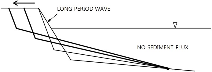
Fig. 9Berm retreat pattern for some net transport at offshore boundary
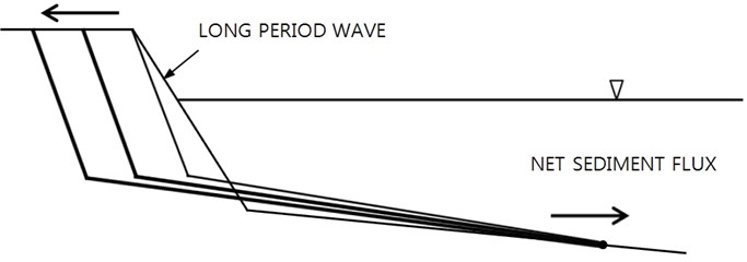
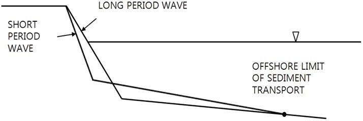
The opposite development is expected for shoreline advance. If the zero-sediment flux condition at the offshore boundary is applied, and the berm area can expand at the onshore boundary, the berm could further be accreted, when long-period waves continue to attack this coast, see Fig. 10. However, the average bed slope in the surf zone gets milder, and eventually berm accretion should stop due to physical limit of the bed slope in the surf zone. If net incoming sediment flux is allowed at the offshore boundary, the berm could then keep on expand forward, see Fig. 11.
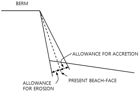
In case the wave climate at a coast is predictable, and the beach-face slopes for possible short wave period and long wave period are known in advance, it would be a good idea to monitor the beach-face slope at the site. If the present beach-face slope is close to the steep slope for short wave period, it could be a warning for serious berm erosion, see Fig. 12. On the other hand, if the present beach-face is close to the mild slope for long wave period, it could be a warning for expansion of the berm crest, if berm crest growth causes any serious problem.
Accuracy of measurement of the beach-face slope is another problem. The equation proposed in the present study is based on the laboratory experiments only, and has not yet been checked against field data. Many other factors may get involved in the problem, and therefore, it is suggested that the beach-face slope at a site may be monitored with wave and tide conditions. The site-specific maximum and minimum beach-face slope at a coast could be used for warning of serious berm erosion or accretion at the site in the future.
Fig. 10Berm accretion pattern for no sediment transport condition across offshore limit
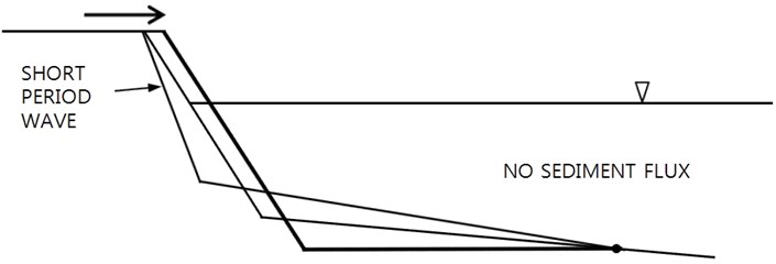
Fig. 11Berm accretion pattern for sediment transport condition across offshore limit
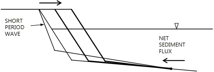
Fig. 12Allowances for erosion and accretion
4. Conclusions
An empirical equation to predict the beach-face slope is proposed here. The independent variables are the wave period, and the bed sediment grain size. Three existing data sets were chosen to extract the coefficients of the equation: one set from a medium-sized flume, and the other two sets from large wave flumes. The coefficients in the equation were obtained from multiple linear regression with two independent variables. The regression results show high correlation coefficient, and are believed to be significant. The absolute power to the wave period in the prediction equation of the beach-face slope is 0.416, while the power to the sediment grain size is 0.122. The new empirical equation shows better agreement to laboratory beach-face slope measurements compared to Sunamura’s and Reis and Gama’s equations.
If the beach-face slope is predictable, it could be used as a sign of future berm erosion or accretion. The shore profile is expressed by two line segments; beach-face, and the rest part of the profile which covers most surf zone. Filtering out detailed bar formation and movement, assuming that an offshore limit exists for sediment transport, expressing the shore profile by two straight lines, the beach-face slope, and the surf zone slope, then the two lines will show interactive changes due to sediment mass conservation. When a storm attacks the area of interest, and the beach-face is adjusting itself to the ongoing storm, the difference between the present beach-face slope and the predicted beach-face slope for short-period waves means the allowance for further beach-face modification with no significant berm erosion. However, if the present beach-face slope is already in the steeper side for short-period waves that means no more allowance is left for safe beach modification, but the berm itself may suffer erosion, which is a serious threat of berm safety for additional future storm. And the opposite situation is also possible. Therefore, it would be important to monitor the beach-face slope at any coastal site to protect future potential berm erosion or accretion.
References
-
O’Connor B. A., Kim H., Yum K. D. Modelling siltation at Chukpyon Harbour, Korea. Computer Modelling of Seas and Coastal Regions, 1992, p. 297-410.
-
Watanabe A., Riho Y., Horikawa K. Beach profiles and on-offshore sediment transport. International Conference on Coastal Engineering, 1980, p. 1106-1121.
-
Kajima R., Shimizu T., Maruyama K., Saito S. Experiments on beach profile change with a large wave flume. International Conference on Coastal Enigineering, 1982, p. 1385-1404.
-
Bailard J. A. Modeling on-offshore sediment transport in the surfzone. International Conference on Coastal Engineering, 1982, p. 1419-1438.
-
Bruun P. Coastal erosion and the development of beach profiles. Technical Memorandum No. 44, Beach Erosion Board, Coastal Engineering Research Center, US Army Engineer Waterways Experiment Station, Vicksburg, MS, 1954.
-
Donnelly C., Kraus N., Larson M. State of knowledge on measurement and modeling of coastal overwash. Journal of Coastal Research, Vol. 22, 2006, p. 965-991.
-
Aagaard T., Black K. P., Greenwood B. Cross-shore suspended sediment transport in the surf zone. Marine Geology, Vol. 185, 2002, p. 283-302.
-
Abreu T., Sancho F., Silva P. A. Generation and evolution of longshore sandbars: model intercomparison and evaluation. Coastal Dynamics, 2013, p. 51-62.
-
Dubarbier B., Castelle B., Marieu V., Michallet H., Grasso F., Ruessink G. Numerical modeling of equilibrium and evolving lightweight sediment laboratory beach profiles. Coastal Dynamics, 2013, p. 521-530.
-
Doering J. C., Bowen A. J. Parametrization of orbital velocity asymmetries of shoaling and breaking waves using bispectral analysis. Coastal Engineering, Vol. 26, Issue 1-2, 1995, p. 15-33.
-
Rakha K. A., Deigaard R. Importance of wave skewness in an intra-wave cross-shore sediment transport model. International Conference on Coastal Engineering, 2000, p. 3179-3192.
-
Doering J. C., Elfrink B., Hanes D. M., Ruessink G. Parameterization of velocity skewness under waves and its effect on cross-shore sediment transport. International Conference on Coastal Engineering, 2000, p. 1383-1396.
-
Sancho F., Abreu T., D’Alessandro F., Tomasicchio G. R., Silva P. A. Surf hydrodynamics in front of collapsing coastal dunes. Journal of Coastal Research, Vol. 64, 2011, p. 144-148.
-
Rocha M., Silva P., Michallet H., Abreu T., Moura D., Moura J. Parameterizations of wave nonlinearity from local wave parameters: a comparison with field data. Journal of Coastal Research, Vol. 65, 2013, p. 374-379.
-
Grasso F., Michallet H., Barthélemy E. Sediment transport associated with morphological beach changes forced by irregular asymmetric, skewed waves. Journal of Geophysical Research, Vol. 116, 2010, p. 1-12.
-
Baldock T. E., Manoonvoravong P., Pham K. S. Sediment transport and beach morphodynamics induced by free long waves, bound long waves and wave groups. Coastal Engineering, Vol. 57, 2010, p. 898-916.
-
Hanson H., Kraus N. C. Genesis: generalized model for simulating shoreline change. CERC Technical Report, CERC-89-19, 1989.
-
Dean R. G. Equilibrium beach profiles: U.S. Atlantic and Gulf coasts. Department of Civil Engineering, Ocean Engineering Report No. 12, University of Delaware, Newark, DE, 1977.
-
Larson M., Kraus N. C. SBEACH: Numerical model for simulating storm-induced beach change. CERC Technical Report, CERC-89-9, 1989.
-
Sunamura T., Horikawa K. Two-dimensional beach transformation due to waves. Proc. 14th International Conference on Coastal Engineering, 1974, p. 920-938.
-
Hoque Md. A., Asano T. Numerical study on wave-induced filtration flow across the beach face. Ocean Engineering, Vol. 34, 2007, p. 2033-2044.
-
Kelly D. M., Dodd N. Beach-face evolution in the swash zone. Journal of Fluid Mechanics, Vol. 661, 2010, p. 316-340.
-
Walgreen M., Swart H. E. D., Calvete D. A model for grain-size sorting over tidal sand ridges. Ocean Dynamics, Vol. 54, 2004, p. 374-384.
-
Sunamura T. Quantitative predictions of beach-face slopes. Geological Society of America Bulletin, Vol. 95, Issue 2, 1984, p. 242-245.
-
Anthony E. J. Sediment-wave parametric characterization of beaches. Journal of Coastal Research, Vol. 14, 1998, p. 347-352.
-
Masselink G., Li L. The role of swash infiltration in determining the beachface gradient: a numerical study. Marine Geology, Vol. 176, 2001, p. 139-156.
-
Reis A. H., Gama C. Sand size versus beachface slope – an explanation based on the constructal law. Geomorphology, Vol. 114, 2010, p. 276-283.
-
Wise R. A., Smith S. J., Larson M. SBEACH: numerical model for simulating storm-induced beach change: Report 4 Cross-shore transport under ramdom waves and model validation with supertank and field data. Coastal Engineering Technical Report CERC-89-9, 1996.
-
Bejan A. Advanced engineering thermodynamics. Second ed., Wiley, New York, 1997.
-
Birkemeier W. Professional development programme: coastal infrastructure design, construction and maintenance: a course in coastal defense system I. Chapter 2: Cross-shore sediment processes, 2001.
-
Lee J. C. Development of survey system of coastal shallow bathymetry. Kiost Internal Report, 2013.
-
Levesque R. SPSS programming and data management: a guide for SPSS and SAS users. Fourth Edition, SPSS Inc., 2007.
About this article
This work has been supported by KIMST as research projects, “Marine and Environmental Prediction System (MEPS)” in 2013, and “Development of Coastal Erosion Control Technology (MIDAS)” in 2014.
