Dynamics and kinematics analysis and simulation of lower extremity power-assisted exoskeleton

Li, Yanbei; Yan, Lei; Qian, Hua; Wu, Jian; Men, Sen; Li, Na

Journal of Vibroengineering

Browse Journal

Submit article

Published: 31 March 2014

Check for updates

Dynamics and kinematics analysis and simulation of lower extremity power-assisted exoskeleton

Yanbei Li¹

Lei Yan²

Hua Qian³

Jian Wu⁴

Sen Men⁵

Na Li⁶

^{1, 2, 3, 4, 5, 6}School of Technology, Beijing Forestry University, China

Corresponding Author:

Lei Yan

Cite the article Download PDF

Downloads 1746

Abstract

According to the walking character of lower extremity power-assisted exoskeleton that was designed by our Robotics Laboratory, D-H convention was applied to the kinematics analysis of this exoskeleton model. Lagrangian dynamics was used to analyzing dynamics for the single-foot support model, double-feet support model and double-feet support with one redundancy model respectively. The kinematical equation was obtained and MATLAB was used to verify its validity. Meanwhile, the kinetic equations and torque of each joint were obtained by virtue of ADAMS. Our study provided a theoretical foundation for the control strategies, and optimization design of the mechanical structure and promoted the practical application of this lower extremity power-assisted exoskeleton in further research.

1. Introduction

Lower extremity power-assisted exoskeleton is a kind of robot which is defined as an electromechanical device in overall or a frame that worn by a human operator. The lower extremity power-assisted exoskeleton is developed mainly to help human perform difficult tasks due to either their physical limitations or muscles’ fatigues. In addition, exoskeletons can increase the endurance, traveling speed, and even balance of the wearer in extremely difficult terrains [1]. With the development of science and technology, the research on lower extremity exoskeleton has gradually extended to the field of mechanics, robotics, bionics, control theory, information processing, and communication technology etc.

As early as in 1960s, our pioneers have started to research on the exoskeleton. A master-slave system named the Hardiman was developed by General Electric in 1968. Furthermore some successful and remarkable examples of lower extremity power-assisted exoskeleton such as BLEEX and HAL, were designed for military missions and power enhancement respectively in the 21st century [2].

The Berkeley Lower Extremity Exoskeleton (BLEEX) project funded by the Defense Advanced Research Project Agency (DARPA), USA, was first unveiled in 2004, at the University of California, Berkeley’s Human Engineering and Robotics Laboratory [3]. It was a field-operational robotic system worn by an operator, which could provide the wearer with the ability of undertaking significant loads on the back with minimal effort when negotiating any terrain. BLEEX featured seven DOFs per leg, and the exoskeleton was actuated via bidirectional linear hydraulic cylinders mounted in a triangular configuration with the rotary joints, resulting in an effective moment arm varying with joint angles [4].

Hybrid Assistive Limb (HAL) was successfully developed in Tsukuba University of Japan which was a lightweight power assist device. The latest model, HAL-5, was a full-body suit unit designed to aid people who had degenerated muscles and paraplegics from brain or spinal injuries. It was connected to thighs and shanks of the patient and moved the patient’s legs as a function of the EMG (electromyogram) signals measured from the wearer [4]. Through the use of DC motors integrated with harmonic drives, each leg of HAL-5 powers the flexion/extension motion at the hip and knee in the sagittal plane.

The lower extremity power-assisted exoskeleton system (LEPES) designed by our Robotics Laboratory is a kind of wearable mechanical legs, which contains mechanical systems, sensors and control systems. The mechanical system includes waist, hip, knee, leg and foot. In regardless of complex activities such as jumping and going-upstairs, the main purpose of LEPES is providing power assistance for wearers when they walk hard. Thus, in the aspect of DOFs’ distribution, the LEPES features three DOFs at the hip, one at the knee, and three at the ankle per leg. Of these, two DOFs are actuated by Maxon DC motors: hip flexion/extension and knee flexion/extension in the sagittal plane. The mechanical structure built in our Robotics Laboratory is shown in Fig. 1.

As a wearable biped exoskeleton system, LEPES should be programmed to walk naturally to provide intimacy to human. However, the human gait is a complex dynamic activity. Therefore, in order to get accurate control strategies and conduct the optimization design of mechanical structure, it is very important and necessary to build the dynamic and kinematics model and gain the kinematical and dynamic equation for LEPES.

Fig. 1The lower extremity power-assisted exoskeleton system

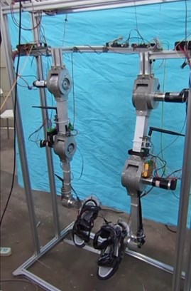
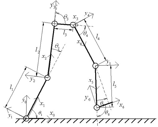
Fig. 2Kinematical model of LEPES

2. Kinematical model of LEPES

The kinematic analysis of LEPES can be facilitated by using the Denavt-Hartenberg (D-H) convention because of its well-established analysis procedures.

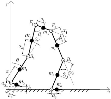
In order to simplify the calculation of the kinematical model, the waist (actually the projection of waist in the sagittal plane), the legs and the feet are regarded as the rigid links; the hip, knee and ankle are simplified as the revolute pair in the sagittal plane. Thus, the whole kinematical model is a five-link biped model, and the link frames ${0}$ through ${6}$ of the LEPES can be established, as shown in Fig. 2. Here, frame ${0}$ represents the world reference frame, where $x_{0}$ is horizontal axis, $y_{0}$ is vertical axis and $z_{0}$ is perpendicular to the surface with the outward direction as the positive direction.

Based on the D-H rules and the five-link biped model, parameters of LEPES can be deduced as shown in Table 1. It should be noted that the parameters in Table 1 can be selected in different ways because the D-H notation is not unique.

According to the D-H convention, D-H homogeneous matrix representation is used to describe the spatial displacement between neighboring link coordinate frames to obtain the information related to kinematics of each link [5].

Assuming ${}^{i - 1}{M_{i}}$ is the homogeneous transformation matrix describing the relative translation and rotation between $l_{i - 1}$ and $l_{i}$ coordinate systems, then we can obtain:

1

{{}^{0}M}_{1} = [\begin{matrix} c θ_{1} & - s θ_{1} & 0 & 0 \\ s θ_{1} & c θ_{1} & 0 & 0 \\ 0 & 0 & 1 & 0 \\ 0 & 0 & 0 & 1 \end{matrix}],

2

{{}^{1}M}_{2} = [\begin{matrix} c θ_{2} & - s θ_{2} & 0 & l_{1} \\ s θ_{2} & c θ_{2} & 0 & 0 \\ 0 & 0 & 1 & 0 \\ 0 & 0 & 0 & 1 \end{matrix}],

3

{{}^{2}M}_{3} = [\begin{matrix} c θ_{3} & - s θ_{3} & 0 & l_{2} \\ s θ_{3} & c θ_{3} & 0 & 0 \\ 0 & 0 & 1 & 0 \\ 0 & 0 & 0 & 1 \end{matrix}],

4

{{}^{3}M}_{4} = [\begin{matrix} c θ_{4} & - s θ_{4} & 0 & l_{3} \\ s θ_{4} & c θ_{4} & 0 & 0 \\ 0 & 0 & 1 & 0 \\ 0 & 0 & 0 & 1 \end{matrix}],

5

{{}^{4}M}_{5} = [\begin{matrix} c θ_{5} & - s θ_{5} & 0 & l_{4} \\ s θ_{5} & c θ_{5} & 0 & 0 \\ 0 & 0 & 1 & 0 \\ 0 & 0 & 0 & 1 \end{matrix}],

6

{{}^{5}M}_{6} = [\begin{matrix} c θ_{6} & - s θ_{6} & 0 & l_{5} \\ s θ_{6} & c θ_{6} & 0 & 0 \\ 0 & 0 & 1 & 0 \\ 0 & 0 & 0 & 1 \end{matrix}],

where $s i n$ and $c o s$ are represented by $s$ and $c$ , respectively.

Table 1D-H parameters for LEPES

$i$	$l_{i - 1}$	$α_{i - 1}$	$d_{i - 1}$	$θ_{i - 1}$	$q_{i}$
0	0	0	0	$θ_{1}$	$θ_{1}$
1	$l_{1}$	0	0	$θ_{2}$	$θ_{2}$
2	$l_{2}$	0	0	$θ_{3}$	$θ_{3}$
3	$l_{3}$	0	0	$θ_{4}$	$θ_{3}$
4	$l_{4}$	0	0	$θ_{5}$	$θ_{5}$
5	$l_{5}$	0	0	$θ_{6}$	$θ_{6}$
Note: $i$ is the link number, $l_{i - 1}$ is the distance between $z_{i - 1}$ and $z_{i}$ along $x_{i}$ , $α_{i - 1}$ is the angle between $z_{i - 1}$ and $z_{i}$ about $x_{i}$ , $d_{i - 1}$ is the distance between $x_{i - 1}$ and $x_{i}$ along $z_{i - 1}$ , $θ_{i}$ is the angle between $x_{i - 1}$ and $x_{i}$ about $z_{i - 1}$ , $q_{i}$ is the joint variable about $l_{i}$ .

Thus, the ankle reference frame ${6}$ can be expressed in the world reference frame ${0}$ , as given in Eq. (7):

7

{{}^{0}M}_{6} = {{}^{0}M}_{1} {{}^{1}M}_{2} {{}^{2}M}_{3} {{}^{3}M}_{4} {{}^{4}M}_{5} {{}^{5}M}_{6} = [\begin{matrix} c \sum_{j = 1}^{6} θ_{j} & - s \sum_{j = 1}^{6} θ_{j} & 0 & l_{5} c \sum_{j = 1}^{5} θ_{j} + l_{4} c \sum_{j = 1}^{4} θ_{j} + l_{3} c \sum_{j = 1}^{3} θ_{j} + l_{2} c \sum_{j = 1}^{2} θ_{j} + l_{1} c θ_{1} \\ s \sum_{j = 1}^{6} θ_{j} & c \sum_{j = 1}^{6} θ_{j} & 0 & l_{5} s \sum_{j = 1}^{5} θ_{j} + l_{4} s \sum_{j = 1}^{4} θ_{j} + l_{3} s \sum_{j = 1}^{3} θ_{j} + l_{2} s \sum_{j = 1}^{2} θ_{j} + l_{1} s θ_{1} \\ 0 & 0 & 1 & 0 \\ 0 & 0 & 0 & 1 \end{matrix}] .

According to D-H convention, Eq. (7) can be transformed as follows:

8

[\begin{matrix} n_{x} & o_{x} & a_{x} & p_{x} \\ n_{y} & o_{y} & a_{y} & p_{y} \\ n_{z} & o_{z} & a_{z} & p_{z} \\ 0 & 0 & 0 & 1 \end{matrix}] = [\begin{matrix} c \sum_{j = 1}^{6} θ_{j} & - s \sum_{j = 1}^{6} θ_{j} & 0 & l_{5} c \sum_{j = 1}^{5} θ_{j} + l_{4} c \sum_{j = 1}^{4} θ_{j} + l_{3} c \sum_{j = 1}^{3} θ_{j} + l_{2} c \sum_{j = 1}^{2} θ_{j} + l_{1} c θ_{1} \\ s \sum_{j = 1}^{6} θ_{j} & c \sum_{j = 1}^{6} θ_{j} & 0 & l_{5} s \sum_{j = 1}^{5} θ_{j} + l_{4} s \sum_{j = 1}^{4} θ_{j} + l_{3} s \sum_{j = 1}^{3} θ_{j} + l_{2} s \sum_{j = 1}^{2} θ_{j} + l_{1} s θ_{1} \\ 0 & 0 & 1 & 0 \\ 0 & 0 & 0 & 1 \end{matrix}] .

Thus, the position of the ankle ${}^{0}{p_{6}}$ can be determined as Eq. (9) with respect to the world reference frame ${0}$ :

9

{{}^{0}p}_{6} = [\begin{matrix} l_{5} c \sum_{j = 1}^{5} θ_{j} + l_{4} c \sum_{j = 1}^{4} θ_{j} + l_{3} c \sum_{j = 1}^{3} θ_{j} + l_{2} c \sum_{j = 1}^{2} θ_{j} + l_{1} c θ_{1} \\ l_{5} s \sum_{j = 1}^{5} θ_{j} + l_{4} s \sum_{j = 1}^{4} θ_{j} + l_{3} s \sum_{j = 1}^{3} θ_{j} + l_{2} s \sum_{j = 1}^{2} θ_{j} + l_{1} s θ_{1} \\ 0 \end{matrix}] .

The posture of the ankle ${}^{0}{R_{6}}$ can be determined as Eq. (10):

10

{{}^{0}R}_{6} = [\begin{matrix} c \sum_{j = 1}^{6} θ_{j} & - s \sum_{j = 1}^{6} θ_{j} & 0 \\ s \sum_{j = 1}^{6} θ_{j} & c \sum_{j = 1}^{6} θ_{j} & 0 \\ 0 & 0 & 1 \end{matrix}] .

3. Dynamic models of LEPES

A human walking gait cycle can be divided into three gait patterns [6]: the single-foot support model(one foot stance, the other swing), double-feet support model(double feet whole stance) and double-feet support with one redundancy model(one foot whole stance while the heel or the toes of the other kicks the ground).

Since the force and the position of center of mass for each leg and each joint are different in each gait pattern, this paper decides to use Lagrangian method to analyze the three gait patterns respectively.

In order to simplify the calculation of the dynamic model, the waist (actually the projection of waist in the sagittal plane), the legs and the feet are regarded as the rigid links; the hip, knee and ankle is simplified as the revolute pair in the sagittal plane.

3.1. The double-feet support model

The double-feet support dynamic model of LEPES is illustrated in Fig. 3, where $α_{i}$ stands for the distance between the center of mass of link $i$ and the ends of link $i$ ; $θ_{i}$ represents the angle between link $i$ and link $i - 1$ ; $l_{i}$ is the length of each link; and $m_{i}$ is the mass of each link $i$ , $i = 1,2,…,6$ ; $B_{1}$ and $B_{2}$ represent the DC motors of knee, $F_{1}$ and $F_{2}$ stands for the DC motors of hip. Coordinate system ${x o y}$ is the world reference frame.

Thus, $G_{i} (x_{i}, y_{i})$ (the center of mass of link $i$ ) can be obtained according to the geometric relationships in Fig. 3:

11

\{\begin{array}{l} x_{0} = a_{0}, \\ x_{1} = a_{1} s θ_{1}, \\ x_{2} = l_{1} s θ_{1} + a_{2} s (θ_{1} - θ_{2}), \\ x_{3} = l_{1} s θ_{1} + l_{2} s (θ_{1} - θ_{2}) + a_{3} s (θ_{3} - θ_{1} + θ_{2}), \\ x_{4} = l_{1} s θ_{1} + l_{2} s (θ_{1} - θ_{2}) + l_{3} s (θ_{3} - θ_{1} + θ_{2}) + a_{4} s (θ_{3} - θ_{1} + θ_{2} - θ_{4}), \\ x_{5} = \{\begin{array}{l} l_{1} s θ_{1} + l_{2} s (θ_{1} - θ_{2}) + l_{3} s (θ_{3} - θ_{1} + θ_{2}) + \\ + l_{4} s (θ_{3} - θ_{1} + θ_{2} - θ_{4}) + a_{5} s (θ_{3} - θ_{1} + θ_{2} - θ_{4} - θ_{5}) \end{array}\}, \\ x_{6} = \{\begin{array}{l} l_{1} s θ_{1} + l_{2} s (θ_{1} - θ_{2}) + l_{3} s (θ_{3} - θ_{1} + θ_{2}) + \\ + l_{4} s (θ_{3} - θ_{1} + θ_{2} - θ_{4}) + l_{5} s (θ_{3} - θ_{1} + θ_{2} - θ_{4} - θ_{5}) + a_{6} \end{array}\}, \end{array}

12

\{\begin{array}{l} y_{0} = 0, \\ y_{1} = a_{1} c θ_{1}, \\ y_{2} = l_{1} c θ_{1} + a_{2} c (θ_{1} - θ_{2}), \\ y_{3} = l_{1} c θ_{1} + l_{2} c (θ_{1} - θ_{2}) - a_{3} c (θ_{3} - θ_{1} + θ_{2}), \\ y_{4} = l_{4} c (θ_{3} - θ_{1} + θ_{2} - θ_{4}) - a_{4} c (θ_{3} - θ_{1} + θ_{2} - θ_{4}) + l_{5} c (θ_{3} - θ_{1} + θ_{2} - θ_{4} - θ_{5}), \\ y_{5} = l_{5} c (θ_{3} - θ_{1} + θ_{2} - θ_{4} - θ_{5}) - a_{5} c (θ_{3} - θ_{1} + θ_{2} - θ_{4} - θ_{5}), \\ y_{6} = 0 . \end{array}

The coordinate of each actuated motor $D_{i} (x_{i}, y_{i})$ is:

13

\{\begin{array}{l} x_{B_{1}} = l_{1} s θ_{1}, \\ x_{F_{1}} = l_{1} s θ_{1} + l_{2} s (θ_{1} - θ_{2}), \\ x_{F_{2}} = l_{1} s θ_{1} + l_{2} s (θ_{1} - θ_{2}) + l_{3} s (θ_{3} - θ_{1} + θ_{2}), \\ x_{B_{2}} = l_{1} s θ_{1} + l_{2} s (θ_{1} - θ_{2}) + l_{3} s (θ_{3} - θ_{1} + θ_{2}) + l_{4} s (θ_{3} - θ_{1} + θ_{2} - θ_{4}), \end{array}

14

\{\begin{array}{l} y_{B_{1}} = l_{1} c θ_{1}, \\ y_{F_{1}} = l_{1} c θ_{1} + l_{2} c (θ_{1} - θ_{2}), \\ y_{F_{2}} = l_{4} c (θ_{3} - θ_{1} + θ_{2} - θ_{4}) + l_{5} c (θ_{3} - θ_{1} + θ_{2} - θ_{4} - θ_{5}), \\ y_{B_{2}} = l_{5} c (θ_{3} - θ_{1} + θ_{2} - θ_{4} - θ_{5}) . \end{array}

Fig. 3The double-feet support model

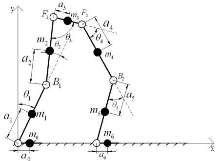
Fig. 4The double-feet support with one redundancy (toes of one foot kicking the ground)

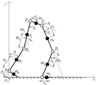
3.2. The double-feet support with one redundancy model

As mentioned above, there are two situations of the double-feet support with one redundancy model, and this study just analyzes the model that one foot whole stances while the toes of the other kick the ground because of the same theories, as shown in Fig. 4.

$α_{i}$ stands for the distance between the center of mass of link $i$ and the ends of link $i$ ; $θ_{i}$ represents the angle between link $i$ and link $i - 1$ ; $l_{i}$ is the length of each link; $m_{i}$ is the mass of each link $i$ , $i =$ 1, 2,…, 6; $B_{1}$ and $B_{2}$ represent the DC motors of knee, $F_{1}$ and $F_{2}$ stands for the DC motors of hip. Coordinate system ${x o y}$ is the world reference frame.

Therefore, $G_{i} (x_{i}, y_{i})$ (the center of mass of link $i$ ) can be obtained according to the geometric relationships:

15

\{\begin{matrix} \begin{array}{l} x_{0} = l_{0} s θ_{0} - a_{0} s θ_{0}, \\ x_{1} = a_{1} s θ_{1}, \\ x_{2} = l_{1} s θ_{1} + a_{2} s (θ_{1} - θ_{2}), \\ x_{3} = l_{1} s θ_{1} + l_{2} s (θ_{1} - θ_{2}) + a_{3} s (θ_{3} - θ_{1} + θ_{2}), \\ x_{4} = l_{1} s θ_{1} + l_{2} s (θ_{1} - θ_{2}) + l_{3} s (θ_{3} - θ_{1} + θ_{2}) + a_{4} s (θ_{3} - θ_{1} + θ_{2} - θ_{4}), \\ x_{5} = \{\begin{array}{l} l_{1} s θ_{1} + l_{2} s (θ_{1} - θ_{2}) + l_{3} s (θ_{3} - θ_{1} + θ_{2}) + l_{4} s (θ_{3} - θ_{1} + θ_{2} - θ_{4}) + \\ + a_{5} s (θ_{3} - θ_{1} + θ_{2} - θ_{4} - θ_{5}) \end{array}\}, \\ x_{6} = \{\begin{array}{l} l_{1} s θ_{1} + l_{2} s (θ_{1} - θ_{2}) + l_{3} s (θ_{3} - θ_{1} + θ_{2}) + l_{4} s (θ_{3} - θ_{1} + θ_{2} - θ_{4}) + \\ + l_{5} s (θ_{3} - θ_{1} + θ_{2} - θ_{4} - θ_{5}) + a_{6} \end{array}\}, \end{array} \end{matrix}

16

\{\begin{array}{l} y_{0} = a_{0} c θ_{0}, \\ y_{1} = a_{1} c θ_{1} + l_{0} c θ_{0}, \\ y_{2} = l_{1} c θ_{1} + a_{2} c (θ_{1} - θ_{2}) + l_{0} c θ_{0}, \\ y_{3} = l_{1} c θ_{1} + l_{2} c (θ_{1} - θ_{2}) - a_{3} c (θ_{3} - θ_{1} + θ_{2}) + l_{0} c θ_{0}, \\ y_{4} = l_{4} c (θ_{3} - θ_{1} + θ_{2} - θ_{4}) - a_{4} c (θ_{3} - θ_{1} + θ_{2} - θ_{4}) + l_{5} c (θ_{3} - θ_{1} + θ_{2} - θ_{4} - θ_{5}), \\ y_{5} = l_{5} c (θ_{3} - θ_{1} + θ_{2} - θ_{4} - θ_{5}) - a_{5} c (θ_{3} - θ_{1} + θ_{2} - θ_{4} - θ_{5}), \\ y_{6} = 0 . \end{array}

The coordinate of each actuated motor $D_{i} (x_{i}, y_{i})$ is:

17

\{\begin{array}{l} x_{B_{1}} = l_{1} s θ, \\ x_{F_{1}} = l_{1} s θ_{1} + l_{2} s (θ_{1} - θ_{2}), \\ x_{F_{2}} = l_{1} s θ_{1} + l_{2} s (θ_{1} - θ_{2}) + l_{3} s (θ_{3} - θ_{1} + θ_{2}), \\ x_{B_{2}} = l_{1} s θ_{1} + l_{2} s (θ_{1} - θ_{2}) + l_{3} s (θ_{3} - θ_{1} + θ_{2}) + l_{4} s (θ_{3} - θ_{1} + θ_{2} - θ_{4}), \end{array}

18

\{\begin{array}{l} y_{B_{1}} = l_{1} c θ_{1} + l_{0} c θ_{0}, \\ y_{F_{1}} = l_{1} c θ_{1} + l_{2} c (θ_{1} - θ_{2}) + l_{0} c θ_{0}, \\ y_{F_{2}} = l_{4} c (θ_{3} - θ_{1} + θ_{2} - θ_{4}) + l_{5} c (θ_{3} - θ_{1} + θ_{2} - θ_{4} - θ_{5}), \\ y_{B_{2}} = l_{5} c (θ_{3} - θ_{1} + θ_{2} - θ_{4} - θ_{5}) . \end{array}

3.3. The single-foot support model

Fig. 5 shows the single-foot support dynamic model of LEPES. $α_{i}$ stands for the distance between the center of mass of link $i$ and the ends of link $i$ ; $θ_{i}$ represents the angle between link $i$ and link $i - 1$ ; $l_{i}$ is the length of each link; $m_{i}$ is the mass of each link $i$ , $i =$ 1, 2,…, 6; $B_{1}$ and $B_{2}$ represent the DC motors of knee, $F_{1}$ and $F_{2}$ stands for the DC motors of hip. Coordinate system ${x o y}$ is the world reference frame.

Thus, $G_{i} (x_{i}, y_{i})$ (the center of mass of link $i$ ) can be obtained according to the geometric relationships:

19

\{\begin{array}{l} x_{0} = l_{0} s θ_{0} - a_{0} s θ_{0}, \\ x_{1} = a_{1} s θ_{1}, \\ x_{2} = l_{1} s θ_{1} + a_{2} s (θ_{1} - θ_{2}), \\ x_{3} = l_{1} s θ_{1} + l_{2} s (θ_{1} - θ_{2}) + a_{3} s (θ_{3} - θ_{1} + θ_{2}), \\ x_{4} = l_{1} s θ_{1} + l_{2} s (θ_{1} - θ_{2}) + l_{3} s (θ_{3} - θ_{1} + θ_{2}) + a_{4} s (θ_{3} - θ_{1} + θ_{2} - θ_{4}), \\ x_{5} = \{\begin{array}{l} l_{1} s θ_{1} + l_{2} s (θ_{1} - θ_{2}) + l_{3} s (θ_{3} - θ_{1} + θ_{2}) + l_{4} s (θ_{3} - θ_{1} + θ_{2} - θ_{4}) + \\ + a_{5} s (θ_{3} - θ_{1} + θ_{2} - θ_{4} - θ_{5}) \end{array}\}, \\ x_{6} = \{\begin{array}{l} l_{1} s θ_{1} + l_{2} s (θ_{1} - θ_{2}) + l_{3} s (θ_{3} - θ_{1} + θ_{2}) + l_{4} s (θ_{3} - θ_{1} + θ_{2} - θ_{4}) + \\ + l_{5} s (θ_{3} - θ_{1} + θ_{2} - θ_{4} - θ_{5}) + a_{6} \end{array}\}, \end{array}

20

\{\begin{array}{l} y_{0} = a_{0} c θ_{0} + h, \\ y_{1} = a_{1} c θ_{1} + l_{0} c θ_{0} + h, \\ y_{2} = l_{1} c θ_{1} + a_{2} c (θ_{1} - θ_{2}) + l_{0} c θ_{0} + h, \\ y_{3} = l_{1} c θ_{1} + l_{2} c (θ_{1} - θ_{2}) - a_{3} c (θ_{3} - θ_{1} + θ_{2}) + l_{0} c θ_{0} + h, \\ y_{4} = l_{4} c (θ_{3} - θ_{1} + θ_{2} - θ_{4}) - a_{4} c (θ_{3} - θ_{1} + θ_{2} - θ_{4}) + l_{5} c (θ_{3} - θ_{1} + θ_{2} - θ_{4} - θ_{5}), \\ y_{5} = l_{5} c (θ_{3} - θ_{1} + θ_{2} - θ_{4} - θ_{5}) - a_{5} c (θ_{3} - θ_{1} + θ_{2} - θ_{4} - θ_{5}), \\ y_{6} = 0 . \end{array}

Fig. 5The single-foot support model

The coordinate of each actuated motor $D_{i} (x_{i}, y_{i})$ is:

21

\{\begin{array}{l} x_{B_{1}} = l_{1} s θ, \\ x_{F_{1}} = l_{1} s θ_{1} + l_{2} s (θ_{1} - θ_{2}), \\ x_{F_{2}} = l_{1} s θ_{1} + l_{2} s (θ_{1} - θ_{2}) + l_{3} s (θ_{3} - θ_{1} + θ_{2}), \\ x_{B_{2}} = l_{1} s θ_{1} + l_{2} s (θ_{1} - θ_{2}) + l_{3} s (θ_{3} - θ_{1} + θ_{2}) + l_{4} s (θ_{3} - θ_{1} + θ_{2} - θ_{4}), \end{array}

22

\{\begin{array}{l} y_{B_{1}} = l_{1} c θ_{1} + l_{0} c θ_{0} + h, \\ y_{F_{1}} = l_{1} c θ_{1} + l_{2} c (θ_{1} - θ_{2}) + l_{0} c θ_{0} + h, \\ y_{F_{2}} = l_{4} c (θ_{3} - θ_{1} + θ_{2} - θ_{4}) + l_{5} c (θ_{3} - θ_{1} + θ_{2} - θ_{4} - θ_{5}), \\ y_{B_{2}} = l_{5} c (θ_{3} - θ_{1} + θ_{2} - θ_{4} - θ_{5}) . \end{array}

3.4. The equation of Lagrangian dynamics

According to the method of Lagrangian dynamics, the Lagrangian function is defined as the difference of the system between kinetic energy $E_{K}$ and potential energy $E_{P}$ , i.e.:

23

L = E_{K} - E_{P} .

The equation of Largrangian dynamics can be obtained according to Eq. (23), as shown in Eq. (24):

24

Q_{j} = \frac{d}{d t} (\frac{\partial L}{\partial {\dot{q}}_{j}}) - \frac{\partial L}{\partial q_{j}}, j = 0,1, . . ., n,

where $n$ is number of generalized coordinate system, $q_{i}$ represents the generalized coordinate, ${\dot{q}}_{j}$ stands for the generalized velocity, $Q_{j}$ is the generalized force or generalized torque applied to the $j$ th coordinate.

The total kinetic energy of drive motors in each dynamics model of LEPES is:

25

E_{I} = \frac{1}{2} (I_{B_{1}} {\dot{q}}_{B_{1}}^{2} + I_{B_{2}} {\dot{q}}_{B_{2}}^{2} + I_{F_{1}} {\dot{q}}_{F_{1}}^{2} + I_{F_{2}} {\dot{q}}_{F_{2}}^{2}),

where ${\dot{q}}_{B_{1}}^{2} = {\dot{x}}_{B_{1}}^{2} + {\dot{y}}_{B_{1}}^{2}$ , ${\dot{q}}_{B_{2}}^{2} = {\dot{x}}_{B_{2}}^{2} + {\dot{y}}_{B_{2}}^{2}$ , ${\dot{q}}_{F_{1}}^{2} = {\dot{x}}_{F_{1}}^{2} + {\dot{y}}_{F_{1}}^{2}$ , ${\dot{q}}_{F_{2}}^{2} = {\dot{x}}_{F_{2}}^{2} + {\dot{y}}_{F_{2}}^{2}$ ; and $I_{B_{1}}$ , $I_{B_{2}}$ , $I_{F_{1}}$ , $I_{F_{2}}$ is equivalent moment of inertia of each motor respectively in generalized coordinate system.

The total kinetic energy of links in each dynamic model of LEPES can be calculated as follows:

26

E_{K} = \sum_{i = 0}^{6} E_{K i},

where $E_{K i} = \frac{1}{2} m_{i} v_{i}^{2}$ , $v_{i}^{2} = {\dot{x}}_{i}^{2} + {\dot{y}}_{i}^{2}$ , $i = 0,1,...,6$ , $m_{i}$ is equivalent mass of each links, $v_{i}$ stands for the velocity of each link in the generalized coordinate.

Thus, the total kinetic energy of each dynamic model of LEPES can be obtained, in accordance with the Eq. (25) and Eq. (26):

27

E_{K I} = E_{K} + E_{I} = \frac{1}{2} (\sum_{i = 0}^{6} m_{i} ({\dot{x}}_{i}^{2} + {\dot{y}}_{i}^{2}) + I_{B_{1}} {\dot{q}}_{B_{1}}^{2} + I_{B_{2}} {\dot{q}}_{B_{2}}^{2} + I_{F_{1}} {\dot{q}}_{F_{1}}^{2} + I_{F_{2}} {\dot{q}}_{F_{2}}^{2}) .

The total potential energy of each dynamic model of LEPES is:

28

E_{P} = \sum_{i = 0}^{6} E_{P i},

where $E_{P i} = m_{i} g y_{i}$ , $g$ is the component of acceleration of gravity along $y$ -axis.

The Lagrangian function for each dynamic model can be expressed as below, based on the Eq. (27) and Eq. (28):

29

L = E_{K I} - E_{P} = \frac{1}{2} (\sum_{i = 0}^{6} m_{i} ({\dot{x}}_{i}^{2} + {\dot{y}}_{i}^{2}) + I_{B_{1}} {\dot{q}}_{B_{1}}^{2} + I_{B_{2}} {\dot{q}}_{B_{2}}^{2} + I_{F_{1}} {\dot{q}}_{F_{1}}^{2} + I_{F_{2}} {\dot{q}}_{F_{2}}^{2}) - \sum_{i = 0}^{6} m_{i} g y_{i} .

Therefore, according to Eq. (24) and Eq. (29), the Lagrange equation of each dynamic model in the $j$ th generalized coordinate can be obtained:

30

Q_{j} = \frac{d}{d t} (\frac{\partial L}{\partial {\dot{θ}}_{j}}) - \frac{\partial L}{\partial θ_{j}} .

Finally, the entire kinetic equation of each dynamics model can be expressed as:

31

Q = {[\begin{matrix} \begin{matrix} \begin{matrix} Q_{0} & Q_{1} \end{matrix} & Q_{2} & Q_{3} \end{matrix} & Q_{4} & Q_{5} \end{matrix}]}^{T} .

In accordance with the Eq. (31), in the double-feet support model, $Q_{0}$ and $Q_{5}$ represented the actuated torque of ankles, $Q_{1}$ and $Q_{4}$ stand for the actuated torque of knees, $Q_{2}$ and $Q_{3}$ are the actuated torque of hips. In the double-feet support with one redundancy model, $Q_{0}$ and $Q_{5}$ represent the actuated torque of ankle that the toes kicking ground and the ankle which the whole foot supporting ground respectively, $Q_{1}$ and $Q_{4}$ stand for the actuated torque of knee that the toes kicking ground and the knee which the whole foot supporting ground respectively, $Q_{2}$ and $Q_{3}$ are the actuated torque of hip that the toes kicking ground and the hip which the whole foot supporting ground respectively. In single-foot support model, $Q_{0}$ and $Q_{5}$ represent as the actuated torque of ankle that the foot swing and the ankle which the foot supporting ground respectively, $Q_{1}$ and $Q_{4}$ stand for the actuated torque of knee that the foot swing and the knee which the foot supporting ground respectively, $Q_{2}$ and $Q_{3}$ are the actuated torque of hip that the foot swing and the hip which the foot supporting ground respectively.

4. Simulations verification

In this Section, MATLAB and ADAMS are used to verify the accuracy of D-H equation of kinematics and Lagrange equation of dynamics respectively.

According to the design principles of exoskeleton mentioned in literature [7], this paper assumes the kinematical parameters of LEPES as listed in Table 2.

Theoretically, according to Eq. (7), the homogeneous transformation matrix can be obtained using the parameters in Table 2:

32

{{}^{0}M}_{6} = [\begin{matrix} 0.87 & - 0.50 & 0 & 759.82 \\ 0.50 & 0.87 & 0 & 119.98 \\ 0 & 0 & 1 & 0 \\ 0 & 0 & 0 & 1 \end{matrix}] .

By virtue of MATLAB, the simulation result of the LEPES’s kinematics model is consistent with the theoretical result, as illustrated in Fig. 6.

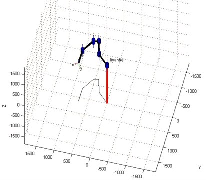
Fig. 6. The simulation result of kinematics model by MATLAB

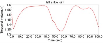
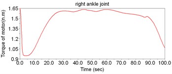
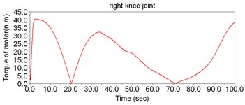
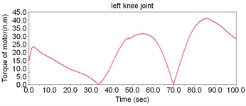
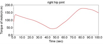
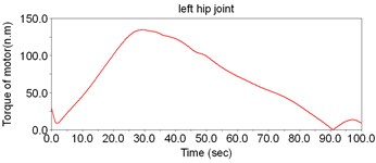
As for the simulation of the dynamic model of LEPES, in order to get the accurate result of dynamics simulation, the data of human gait mentioned in literature [8] and ADAMS are used. Fig. 7 shows the virtual prototype of the LEPES’s dynamic model built by ADAMS, and the torques of actuated motors can be obtained by the simulation, as shown in Fig. 8.

Table 2The given kinematical parameters of LEPES

Link	Length	Joint variable	Angle
$l_{1}$	420 mm	$q_{1}$	$- \frac{π}{4}$
$l_{2}$	419 mm	$q_{2}$	$- \frac{π}{6}$
$l_{3}$	200 mm	$q_{3}$	$\frac{π}{2}$
$l_{4}$	419mm	$q_{4}$	$\frac{π}{4}$
$l_{5}$	420 mm	$q_{5}$	$\frac{π}{6}$
		$q_{6}$	$- \frac{π}{3}$

According to Fig. 8, the motor torque of the hip joint is the largest, while the torque of ankle is the smallest. Thus, there is no need to set motors to drive the ankles; instead, the DOFs of ankles can be regarded as the assistant DOFs when designing the structure.

Fig. 7The virtual prototype of LEPES’s dynamics model

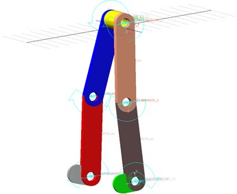
Fig. 8The simulation result of dynamic model of LEPES

a)

b)

c)

d)

e)

f)

5. Conclusions

In conclusion, from kinematical views of the lower extremity power-assisted exoskeleton system which is designed by our Robotic Laboratory, this paper described the kinematical characteristics of the lower extremity power-assisted exoskeleton system (LEPES) via Denavt-Hartenberg (D-H) convention, and the homogeneous transformation matrix that could describe the position and posture of the kinematical model of LEPES was obtained. Thus, the precise position and gesture of the end ankle could be obtained according to the kinematical equation and the $θ_{i}$ ( $i = 1, 2,..., 6$ ) given by the further researches which put forward an improved control strategies. Therefore, this research on kinematics provided a significant theoretical basis for the further study on control strategies and control algorithm of the actuated motors.

In addition, as for the dynamic analysis, Largrangian dynamics was applied to get the kinetic equations of the three dynamic models of LEPES. And the kinetic equation of each model is obtained. According to the Largrangian dynamics of LEPES, the theoretical torque of each motor in each model could be calculated, which was helpful to choosing the drive motors of LEPES and optimizing the whole structure. Therefore, this research on dynamics provided an essential theoretical basis for the motor selection and the optimization design of mechanical structure.

References

Narong Aphiratsakun, Kittipat Chairungsarpsook, Manukid Parnichkun ZMP based gait generation of AIT’s leg exoskeleton. IEEE, 2010.

Search CrossRef
Narong Aphiratsakun, Manukid Parnichkun Fuzzy based gains tuning of PD controller for joint position control of AIT leg exoskeleton-I (ALEX-I). International Conference on Robotics and Biomimetics, Proceedings of the IEEE, 2008.

Search CrossRef
Zhang Sheng, Zhang Hu Simulation of exoskeleton’s virtual joint torque control. International Conference on Advanced Computer Science and Electronics Information, 2013.

Search CrossRef
Aaron M. Dollar, Aaron M. Dollar Lower extremity exoskeletons and active orthoses: challenges and state-of-the-art. IEEE Transactions on Robotics, Vol. 24, Issue 1, 2008, p. 1-15.

Search CrossRef
Shibendu Shekhar Roy, Dilip Kumar Pratihar Kinematics, dynamics and power consumption analyses for turning motion of a six-legged robot. J. Intell. Robot. Syst., 2013.

Search CrossRef
Yali Han, Xingsong Wang Dynamic analysis and simulation of lower limb power-assisted exoskeleton. Journal of System Simulation, Vol. 25, Issue 1, 2013.

Search CrossRef
Jiafan Zhang, Ying Chen, Canjun Yang Human intelligence system and flexible exoskeleton. Science Press, 2011.

Search CrossRef
Maojun Yin Analysis and design of wearable lower extremity exoskeleton. Beijing University of Technology, 2010.

Search CrossRef
Bing Lei Structure optimization and performance evaluation of leg exoskeleton for load-carrying augment. East China University of Science and Technology, 2011.

Search CrossRef
Jianbo Wu Research on spatial forces mechanisms of lower assistant robotic. East China University of Science and Technology, 2012.

Search CrossRef
Yanbao Wu, Yong Yu, Dezhang Xu, Zhongcheng Wu, Feng Chen Kinematics analysis and simulation of a robot with wearable and power-assisted lower extremities. Mechanical Science and Technology, Vol. 25, Issue 2, 2007, p. 235-240.

Search CrossRef
Feng Chen, Min Tang, Weiguo Ma, Xianfei Liu Dynamics analysis and application of the rehabilitation power assist robot for the leg. Journal of Clinical Rehabilitative Tissue Engineering Research, Vol. 15, Issue 30, 2011, p. 5518-5521.

Search CrossRef
Byoung Gook Loh, Jacob Rosen Kinematic analysis of 7 degrees of freedom upper-limb exoskeleton robot with tilted shoulder abduction. International Journal of Precision Engineering and Manufacturing, Vol. 14, Issue 1, 2013, p. 69-76.

Search CrossRef
Wisama Khalil, Ouarda Ibrahim General solution for the dynamic modeling of parallel robots. Journal ofIntelligent and Robotic Systems, Vol. 49, 2007, p. 19-37.

Search CrossRef
Yangmin Li, Qingsong Xu Kinematic analysis and design of a new 3-DOF translational parallel manipulator. Journal of Mechanical Design, Vol. 128, 2006, p. 729-737.

Search CrossRef
Duy Khoa Le, Thanh Liem Dao, Kyoung Kwan Ahn Inverse kinematic analysis for 7-DOF redundant power assistant robot control. 16th International Conference on Mechatronics Technology, 2012, p. 376-381.

Search CrossRef

About this article

Received

13 November 2013

Accepted

23 January 2014

Published

31 March 2014

Keywords

lower exoskeleton

dynamic

kinematics

simulation

Acknowledgements

This research was financially supported by the Fundamental Research Funds for the Central Universities (TD2013-3). The authors also appreciate very much the comments and suggestions from anonymous reviewers and the editors.

This is an open access article distributed under the Creative Commons Attribution License, which permits unrestricted use, distribution, and reproduction in any medium, provided the original work is properly cited.