Stability and local bifurcation analysis for a nonlinear coupled helicopter blade-absorber system via normal form method

Zhou, Wei; Han, Jinglong

Journal of Vibroengineering

Browse Journal

Submit article

Published: 31 March 2014

Check for updates

Stability and local bifurcation analysis for a nonlinear coupled helicopter blade-absorber system via normal form method

Wei Zhou¹

Jinglong Han²

^{1, 2}State Key Laboratory of Mechanics and Control of Mechanical Structures Nanjing University of Aeronautics and Astronautics, Nanjing, 210016, China

Corresponding Author:

Wei Zhou

Cite the article Download PDF

Downloads 1166

Abstract

Consider the effect of nonlinear spring and linear viscous damping in structure, the motion equations of a helicopter blade-absorber system has been established by Lagrange equation. Since the helicopter blade-absorber system exists motion coupling, the inertia and stiffness terms of equations are decoupled via equivalent principal coordinate transformation. The stability and local bifurcation behaviors of the principal coordinate equations are investigated with the aid of multiple scales method and normal form theory. Two kinds of critical points for the bifurcation response equations near the combination resonance are considered, which are characterized by a pair of purely imaginary eigenvalues and double zero eigenvalues. The Hopf bifurcation solution, bifurcation path, and transition curves of the model are investigated respectively. For each case, the numerical results obtained by Runge-Kutta method coincide with the analytical predictions. These results may provide some guidance for parameter design of helicopter blade-absorber system.

1. Introduction

Normal form method is one of the basic methods in the study of nonlinear vibration. The essential idea of the normal form method is using successive coordinate transformations to systematically establish the simplest possible form of the original differential equations. The simple form can demonstrate all possible dynamical properties of the original system in the neighborhood of the bifurcation point. Normal forms are generally not uniquely defined, and finding a normal form for a given system of differential equations is not a simple task. In recent years, normal form methods have got much development. Among them, Yu et al. have proposed and improved a normal form method with a combination of perturbation analysis and computer algebra in [1-8]. Since the reduced system obtained by this normal form method can be more convenient to study bifurcation and stability, Zhang [9] studied the local bifurcation of a nonlinear viscoelastic panel in supersonic flow model via this method, which is characterized by a pair of purely imaginary eigenvalues. Subsequently, she and coauthors researched the stability and local bifurcation of functionally graded material plate under transversal and in-plane excitations in [10]. In addition, Zhou et al. studied several dynamical behaviors for a two degrees of freedom pitch-roll ship via this normal form method in [11]. Wang et al. [12] research on the stability and bifurcation for a flexible beam under a large linear motion with a combination parametric resonance.

Vibration problem has always restricted the development of helicopter, and it is also an important problem which scholars have been dedicated to research and solve. During flight, there are many factors leading to helicopter vibration. In particular, blade flapping, lagging and aerodynamical action can make a significant rotor vibration, meanwhile, fuselage vibration transfers along hub and interacts with rotor, which will aggravate overall vibration. In order to reduce the vibration level of helicopter blade and fuselage, people take a method of setting absorber on blade or hub. For instance, absorbers installed on Boeing Vertol 347, Lynx and Black Hawk have been achieved satisfactory effects [13, 14]. However, if absorber parameters are designed unreasonable, not only may generate resonance phenomenon, but also may cause entire system instability or even leading to a disastrous consequences [15, 16]. Therefore, the research on helicopter blade-absorber system dynamics behavior is of important theoretical and practical significance.

Helicopter blade-absorber system not only contains complex nonlinear structure but also exists motion coupling between each degrees of freedom, therefore, its mathematical modeling and theoretical analysis both have certain difficulties. At present, the research on this system usually adopts experiment or numerical simulation [17-20]. Since the analysis objects of analytic method generally can not be too complicated, the qualitative study on helicopter blade-absorber system is relatively rare [13, 21, 22]. Among them, Nagasaka et al. [21, 22] respectively established two degrees of freedom blade-absorber and three degrees of freedom blade-absorber-fuselage model, numerical simulated the vibration response and verified the numerical results by van der Pol method. However, in the above two models, only linear structure is considered, and it is obviously not enough for the in-depth study on dynamical behaviors.

In view of the above problems, in this paper the normal form method proposed by Yu will be first introduced to the dynamics analysis of helicopter blade-absorber system, also, at modeling time, structure nonlinear will be considered. Firstly, establish a helicopter blade-absorber model by Lagrange equation. As the helicopter blade-absorber system exists motion coupling, the inertia and stiffness terms of equations are decoupled via equivalent principal coordinate transformation. The stability and local bifurcation behaviors of the principal coordinate equations are investigated with the aid of multiple scales method and normal form theory. Two kinds of degenerated equilibrium points of the bifurcation response equations are considered, which are characterized by a pair of purely imaginary eigenvalues and a pair of complex conjugate having negative real part as well as a double zero eigenvalues. Finally, Hopf bifurcation solution, bifurcation path and transition curves are obtained. The analytical predictions agree with the results of Runge-Kutta method.

This paper is organized as follows: in Section 2, a helicopter blade-absorber model is established. In Section 3, the bifurcation response equations near combination resonance are obtained using multiple scales method. The detailed stability and local bifurcation analysis of the bifurcation response equations in the vicinity of the critical points are given in Section 4, which is followed in Section 5 by a short conclusion.

2. Helicopter blade-absorber modeling

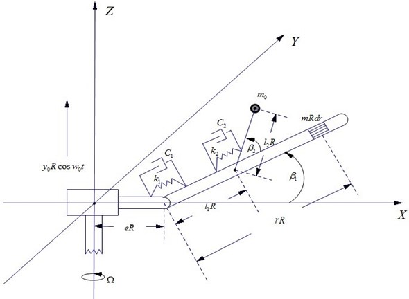
This paper focuses on the stability and local bifurcation behaviors of a helicopter blade-absorber system. Consider pendulum absorber is designed in helicopter blade flapping direction, and there is a harmonic excitation $y_{0} R c o s ω_{0} t$ acting on rotor hub position. The connections of blade-hub and blade-absorber are simplified as damping and elastic hinge restrictions. The horizontal displacement of hub is omitted. The blade-absorber system physical model is shown in Fig. 1. Aerodynamic force model adopts blade micro segment aerodynamic force $Ω^{2} F_{b} c o s ω_{1} t$ , which can be found in [22].

Take blade flapping angle $β_{1}$ and absorber swinging angle (relative to the blade) $β_{2}$ as generalized coordinate. Let upward direction is positive. The coordinate of blade micro segment $m R d r$ on the $r R$ position is:

1

x_{1} = (e + r c o s β_{1}) R,

2

z_{1} = (r s i n β_{1} + y_{0} c o s ω_{0} t) R .

If blade rotates with angular velocity $Ω$ , then its velocity in $Y$ direction is:

3

{\dot{y}}_{1} = x Ω .

Fig. 1Physical model of a helicopter blade-absorber system

The coordinate of absorber mass $m_{0}$ is:

4

x_{2} = [e + l_{1} c o s β_{1} + l_{2} c o s (β_{1} + β_{2})] R,

5

z_{2} = [l_{1} s i n β_{1} + l_{2} s i n (β_{1} + β_{2}) + y_{0} c o s ω_{0} t] R .

It has $Y$ direction velocity:

6

{\dot{y}}_{2} = x Ω .

Using Lagrange equation and small angle assumption, blade-absorber system flapping motion equations can be obtained as follows:

7

R^{2} [\frac{1}{3} {(1 - e)}^{3} m R + {(l_{1} + l_{2})}^{2} m_{0}] {\ddot{β}}_{1} + R^{2} l_{2} m_{0} (l_{1} + l_{2}) {\ddot{β}}_{2} + Ω^{2} R^{2} \{[\frac{1}{2} {(1 - e)}^{2} e + \frac{1}{3} {(1 - e)}^{3}] m R + [{(l_{1} + l_{2})}^{2} + e (l_{1} + l_{2})] m_{0}\} β_{1} + Ω^{2} R^{2} l_{2} m_{0} (e + l_{1} + l_{2}) β_{2} + k_{1} (β_{1}) + c_{1} ({\dot{β}}_{1}) = R^{2} ω_{0}^{2} y_{0} c o s (ω_{0} t) \cdot [\frac{1}{2} {(1 - e)}^{2} m R + (l_{1} + l_{2}) m_{0}] + R^{2} Ω^{2} F_{b} c o s (ω_{1} t) (1 - e),

8

R^{2} l_{2} m_{0} (l_{1} + l_{2}) {\ddot{β}}_{1} + R^{2} l_{2}^{2} m_{0} {\ddot{β}}_{2} + Ω^{2} R^{2} l_{2} m_{0} (e + l_{1} + l_{2}) β_{1} + Ω^{2} R^{2} l_{2} m_{0} (e + l_{1} + l_{2}) β_{2} + k_{2} (β_{2}) + c_{2} ({\dot{β}}_{2}) = l_{2} m_{0} R^{2} ω_{0}^{2} y_{0} c o s (ω_{0} t),

where $k_{1} (β_{1}),$ $k_{2} (β_{2}),$ $c_{1} ({\dot{β}}_{1}),$ $c_{2} ({\dot{β}}_{2})$ are blade-absorber hinge-spring and hinge-damping constitutive relation respectively. For linear viscous damper and weak nonlinear spring condition, there are:

9

c_{1} ({\dot{β}}_{1}) = ε c_{1}^{'} {\dot{β}}_{1}, c_{2} ({\dot{β}}_{2}) = ε c_{2}^{'} {\dot{β}}_{2},

10

k_{1} (β_{1}) = k_{1} β_{1} + ε k_{2} β_{1}^{2} + ε k_{3} β_{1}^{3}, k_{2} (β_{2}) = k_{4} β_{2} + ε k_{5} β_{2}^{2} + ε k_{6} β_{2}^{3},

where $ε$ is a small parameter and $ε > 0$ .

Supposing $ω_{0} = ω_{1} = Ω$ , $ψ = Ω t$ , and applying dimensionless method, Eq. (7) and (8) can be simplified as follows:

11

β_{1}^{''} + a_{1} β_{1}^{''} + ω_{1}^{2} β_{1} + b_{1} β_{2} + ε (c_{1} β_{1}^{'} + d_{1} β_{1}^{2} + e_{1} β_{1}^{3}) = f_{1} c o s (ω ψ),

12

β_{2}^{''} + a_{2} β_{2}^{''} + b_{2} β_{1} + ω_{2}^{2} β_{2} + ε (c_{2} β_{2}^{'} + d_{2} β_{2}^{2} + e_{2} β_{2}^{3}) = f_{2} c o s (ω ψ),

where $a_{1} = l_{2} (l_{1} + l_{2}) γ Δ$ , $b_{1} = l_{2} γ (e + l_{1} + l_{2}) Δ$ , $c_{1} = 2 η_{1} ω_{β_{1}} / [1 + 3 {(l_{1} + l_{2})}^{2} γ / {(1 - e)}^{3}]$ , $d_{1} = \frac{k_{2} γ}{Ω^{2} R^{3} m}$ , $e_{1} = \frac{k_{3} Δ}{Ω^{2} R^{3} m}$ , $f_{1} = \{[\frac{1}{2} {(1 - e)}^{2} + (l_{1} + l_{2}) γ] y_{0} + F_{b} (1 - e)\} ω^{2} Δ$ ,

$ω_{1} = \sqrt{\{\frac{1}{2} {(1 - e)}^{2} e + \frac{1}{3} {(1 - e)}^{3} + [{(l_{1} + l_{2})}^{2} + e (l_{1} + l_{2})] σ\} \cdot γ + \frac{ω_{β_{1}}^{2}}{[1 + 3 {(l_{1} + l_{2})}^{2} γ / {(1 - e)}^{3}]}}$ ,

$a_{2} = 1 + \frac{l_{1}}{l_{2}}$ , $b_{2} = 1 + \frac{e}{l_{2}} + \frac{l_{1}}{l_{2}}$ , $ω_{2} = \sqrt{1 + \frac{e}{l_{2}} + \frac{l_{1}}{l_{2}} + ω_{β_{2}}^{2}}$ , $c_{2} = 2 η_{2} ω_{β_{2}}$ , $d_{2} = \frac{k_{5}}{Ω^{2} R^{2} l_{2}^{2} m_{0}}$ ,

$e_{2} = \frac{k_{6}}{Ω^{2} R^{2} l_{2}^{2} m_{0}}$ , $f_{2} = \frac{ω^{2} y_{0}}{l_{2}}$ . Among them, $γ = \frac{m_{0}}{m R}$ , $ω = \frac{ω_{0}}{Ω}$ , $Δ = \frac{1}{\frac{1}{3} {(1 - e)}^{3} + {(l_{1} + l_{2})}^{2} γ}$ ,

$I_{b} = \frac{1}{3} {(1 - e)}^{3} m R^{3}$ , $ω_{β_{1}} = \sqrt{\frac{k_{1}}{Ω^{2} I_{b}}}$ , $η_{1} = \frac{c_{1}^{'}}{2 Ω ω_{β_{1}} I_{b}}$ , $ω_{β_{2}} = \sqrt{\frac{k_{4}}{Ω^{2} R^{2} l_{2}^{2} m_{0}}}$ , $η_{2} = \frac{c_{2}^{'}}{2 Ω ω_{β_{2}} R^{2} l_{2}^{2} m_{0}}$ .

In order to decouple the inertia and elastic terms in Eq. (11) and Eq. (12), we use coordinate transformations:

13

(\begin{matrix} β_{1} \\ β_{2} \end{matrix}) = Q (\begin{matrix} x_{1} \\ x_{2} \end{matrix}),

where $x_{1}$ , $x_{2}$ are the principal coordinates of undamped derivation system and $Q = (\begin{matrix} 1 & 1 \\ q_{21} & q_{22} \end{matrix})$ .

q_{21} = - \frac{ω_{1}^{2} - \frac{- a_{2} b_{1} - a_{1} b_{2} + ω_{1}^{2} + ω_{2}^{2} - \sqrt{{(a_{2} b_{1} + a_{1} b_{2} - ω_{1}^{2} - ω_{2}^{2})}^{2} - 4 (1 - a_{1} a_{2}) (- b_{1} b_{2} + ω_{1}^{2} ω_{2}^{2})}}{2 (1 - a_{1} a_{2})}}{b_{1} - \frac{a_{1} (- a_{2} b_{1} - a_{1} b_{2} + ω_{1}^{2} + ω_{2}^{2} - \sqrt{{(a_{2} b_{1} + a_{1} b_{2} - ω_{1}^{2} - ω_{2}^{2})}^{2} - 4 (1 - a_{1} a_{2}) \sqrt{- b_{1} b_{2} + ω_{1}^{2} ω_{2}^{2}}})}{2 (1 - a_{1} a_{2})}},

q_{22} = - \frac{ω_{1}^{2} - \frac{- a_{2} b_{1} - a_{1} b_{2} + ω_{1}^{2} + ω_{2}^{2} - \sqrt{{(a_{2} b_{1} + a_{1} b_{2} - ω_{1}^{2} - ω_{2}^{2})}^{2} - 4 (1 - a_{1} a_{2}) (- b_{1} b_{2} + ω_{1}^{2} ω_{2}^{2})}}{2 (1 - a_{1} a_{2})}}{b_{1} - \frac{a_{1} (- a_{2} b_{1} - a_{1} b_{2} + ω_{1}^{2} + ω_{2}^{2} + \sqrt{{(a_{2} b_{1} + a_{1} b_{2} - ω_{1}^{2} - ω_{2}^{2})}^{2} - 4 (1 - a_{1} a_{2}) \sqrt{- b_{1} b_{2} + ω_{1}^{2} ω_{2}^{2}}})}{2 (1 - a_{1} a_{2})}} .

Then the original equations Eq. (11) and Eq. (12) can be transformed into equivalent principal coordinate equations with inertia and elastic decoupling as:

14

x_{1}^{''} + ω_{n_{1}}^{2} x_{1} = ε (- γ_{1} x_{1}^{'} + γ_{2} x_{2}^{'} + μ_{1} x_{1}^{2} + μ_{2} x_{1} x_{2} + μ_{3} x_{2}^{2} + v_{1} x_{1}^{3} + v_{2} x_{1}^{2} x_{2}

+ v_{3} x_{1} x_{2}^{2} + v_{4} x_{2}^{3}) + p_{1} c o s (ω ψ),

15

x_{2}^{''} + ω_{n_{2}}^{2} x_{2} = ε (γ_{3} x_{1}^{'} - γ_{4} x_{2}^{'} + μ_{4} x_{1}^{2} + μ_{5} x_{1} x_{2} + μ_{6} x_{2}^{2} + v_{5} x_{1}^{3} + v_{6} x_{1}^{2} x_{2}

+ v_{7} x_{1} x_{2}^{2} + v_{8} x_{2}^{3}) + p_{2} c o s (ω ψ),

where:

ω_{n_{1}, n_{2}}^{2} = \frac{1}{2 (1 - a_{1} a_{2})} [\begin{matrix} ω_{1}^{2} + ω_{2}^{2} - a_{1} b_{2} - a_{2} b_{1} \\ \pm \sqrt{{(ω_{1}^{2} + ω_{2}^{2} - a_{1} b_{2} - a_{2} b_{1})}^{2} - 4 (1 - a_{1} a_{2}) (ω_{1}^{2} ω_{2}^{2} - b_{1} b_{2})} \end{matrix}] .

Since the other coefficients of Eq. (14) and Eq. (15) are too complex, using symbols instead of them, and the specific forms are omitted here.

3. Combination resonance analysis

Utilizing multiple scales method, the first-order approximate solution of Eq. (14) and Eq. (15) can be expanded as:

16

x_{i} (ψ, ε) = x_{i 0} (T_{0}, T_{1}) + ε x_{i 1} (T_{0}, T_{1}), i = 1, 2,

where $T_{0} = ψ$ is fast variable, and $T_{1} = ε ψ$ is slow variable. Suppose:

17

\frac{d}{d ψ} = \frac{\partial}{\partial T_{0}} \frac{d T_{0}}{d ψ} + \frac{\partial}{\partial T_{1}} \frac{d T_{1}}{d ψ} = D_{0} + ε D_{1},

18

\frac{d}{d ψ} = \frac{\partial}{\partial T_{0}} \frac{d T_{0}}{d ψ} + \frac{\partial}{\partial T_{1}} \frac{d T_{1}}{d ψ} = D_{0} + ε D_{1} .

Applying the relation of Eq. (17) and Eq. (18), we obtain:

19

\{\begin{array}{l} D_{0}^{2} x_{10} + ω_{n_{1}}^{2} x_{10} = p_{1} c o s (ω ψ), \\ D_{0}^{2} x_{20} + ω_{n_{2}}^{2} x_{20} = p_{2} c o s (ω ψ), \end{array}

20

\{\begin{array}{l} D_{0}^{2} x_{11} + ω_{n_{1}}^{2} x_{11} = (\begin{array}{l} - 2 D_{0} D_{1} x_{10} - γ_{1} D_{0} x_{10} + γ_{2} D_{0} x_{20} + μ_{1} x_{10}^{2} + μ_{2} x_{10} x_{20} \\ + μ_{3} x_{20}^{2} + v_{1} x_{10}^{3} + v_{2} x_{10}^{2} x_{20} + v_{3} x_{10} x_{20}^{2} + v_{4} x_{20}^{3} \end{array}), \\ D_{0}^{2} x_{21} + ω_{n_{2}}^{2} x_{21} = (\begin{array}{l} - 2 D_{0} D_{1} x_{20} + γ_{3} D_{0} x_{10} - γ_{4} D_{0} x_{20} + μ_{4} x_{10}^{2} + μ_{5} x_{10} x_{20} \\ + μ_{6} x_{20}^{2} + v_{5} x_{10}^{3} + v_{6} x_{10}^{2} x_{20} + v_{7} x_{10} x_{20}^{2} + v_{8} x_{20}^{3} \end{array}) . \end{array}

The solutions of zero-order approximate Equation (19) can be expressed as:

21

x_{10} = A_{1} (T_{1}) e x p (i ω_{n_{1}} T_{0}) + B_{1} e x p (i ω T_{0}) + c c,

22

x_{20} = A_{2} (T_{1}) e x p (i ω_{n_{2}} T_{0}) + B_{2} e x p (i ω T_{0}) + c c,

where $A_{i}$ is plural form free vibration amplitude, and $B_{i}$ is real form forced vibration amplitude, $B_{i} = \frac{p_{i}}{2 (ω_{n_{i}}^{2} - ω^{2})}$ , $i = 1, 2$ . $c c$ represents the conjugate term of all the previous terms.

Substitute zero-order approximate solutions (21) and (22) into first-order Eq. (20). By frequency combination relation $ω = ω_{n_{1}} + ω_{n_{2}} + ε σ$ ( $σ$ is a tuning parameter), secular terms can be eliminated. We obtain the following equations with respect to $A_{1}$ , $A_{2}$ :

23

- 2 i ω_{n_{1}} A_{1}^{'} - γ_{1} i ω_{n_{1}} A_{1} + 2 v_{3} A_{1} A_{2} {\bar{A}}_{2} + 6 v_{1} A_{1} B_{1}^{2} + 3 v_{1} A_{1}^{2} {\bar{A}}_{1} + 4 v_{2} A_{1} B_{1} B_{2}

+ 2 v_{3} A_{1} B_{2}^{2} + (μ_{2} {\bar{A}}_{2} B_{1} + 2 μ_{3} {\bar{A}}_{2} B_{2}) e x p (i σ T_{1}) = 0

24

- 2 i ω_{n_{2}} A_{2}^{'} - γ_{4} i ω_{n_{4}} A_{2} + 2 v_{6} A_{1} A_{2} {\bar{A}}_{1} + 6 v_{8} A_{2} B_{2}^{2} + 3 v_{8} A_{2}^{2} {\bar{A}}_{2} + 4 v_{7} A_{2} B_{1} B_{2}

+ 2 v_{6} A_{2} B_{1}^{2} + (μ_{5} {\bar{A}}_{1} B_{2} + 2 μ_{4} {\bar{A}}_{1} B_{1}) e x p (i σ T_{1}) = 0

where ${()}^{'} = \frac{d}{d T_{1}}$ and $\bar{()}$ represents conjugated term. From the process of eliminating secular terms, it can be seen that when using multiple scales method to investigate nonlinear effect on motion characteristics of blade-absorber system, only combination resonance in $ω \approx ω_{n_{1}} + ω_{n_{2}}$ case can be considered.

Suppose $A_{1} (T_{1}) = (g_{r 1} + i g_{i 1}) e x p (\frac{1}{2} i σ T_{1})$ , $A_{2} (T_{1}) = (g_{r 2} + i g_{i 2}) e x p (\frac{1}{2} i σ T_{1})$ , where $g_{r 1}$ , $g_{i 1}$ , $g_{r 2}$ and $g_{i 2}$ are all real number. Substituting $A_{1}$ and $A_{2}$ into Eq. (23), (24) yields:

25

g_{r 1}^{'} = - \frac{γ_{1}}{2} g_{r 1} + (\frac{σ}{2} + \frac{L}{ω_{n_{1}}}) g_{i 1} - \frac{K}{2 ω_{n_{1}}} g_{i 2} + \frac{3 v_{1}}{2 ω_{n_{1}}} g_{i 1} (g_{i 1}^{2} + g_{r 1}^{2}) + \frac{v_{3}}{ω_{n_{1}}} g_{i 1} (g_{r 2}^{2} + g_{i 2}^{2}),

26

g_{i 1}^{'} = - (\frac{σ}{2} + \frac{L}{ω_{n_{1}}}) g_{r 1} - \frac{γ_{1}}{2} g_{i 1} - \frac{K}{2 ω_{n_{1}}} g_{r 2} - \frac{3 v_{1}}{2 ω_{n_{1}}} g_{i 1} (g_{i 1}^{2} + g_{r 1}^{2}) - \frac{v_{3}}{ω_{n_{1}}} g_{i 1} (g_{r 2}^{2} + g_{i 2}^{2}),

27

g_{r 2}^{'} = - \frac{M}{2 ω_{n_{2}}} g_{i 1} - \frac{γ_{4}}{2} g_{r 2} + (\frac{σ}{2} + \frac{N}{ω_{n_{2}}}) g_{i 2} + \frac{3 v_{8}}{2 ω_{n_{2}}} g_{i 2} (g_{r 2}^{2} + g_{i 2}^{2}) + \frac{v_{6}}{ω_{n_{2}}} g_{i 2} (g_{r 1}^{2} + g_{i 1}^{2}),

28

g_{i 2}^{'} = - \frac{M}{2 ω_{n_{2}}} g_{r 1} - (\frac{σ}{2} + \frac{N}{ω_{n_{2}}}) g_{r 2} - \frac{γ_{4}}{2} g_{i 2} - \frac{3 v_{8}}{2 ω_{n_{2}}} g_{r 2} (g_{r 2}^{2} + g_{i 2}^{2}) - \frac{v_{6}}{ω_{n_{2}}} g_{i 2} (g_{r 1}^{2} + g_{i 1}^{2}),

where $K = μ_{2} B_{1} + 2 μ_{3} B_{2},$ $L = 2 v_{2} B_{1} B_{2} + 3 v_{1} B_{1}^{2} + v_{3} B_{2}^{2},$ $N = 2 v_{7} B_{1} B_{2} + 3 v_{8} B_{2}^{2} + v_{6} B_{1}^{2},$ $M = μ_{5} B_{2} + 2 μ_{4} B_{1}$ .

The Jacobi matrix of system (25) to (28) on the initial equilibrium solution $(g_{r 1}, g_{i 1}, g_{r 2}, g_{i 2}) = (0,0, 0,0)$ is:

29

J = [\begin{matrix} - \frac{γ_{1}}{2} & \frac{σ}{2} + \frac{L}{ω_{n_{1}}} & 0 & - \frac{K}{2 ω_{n_{1}}} \\ - (\frac{σ}{2} + \frac{L}{ω_{n_{1}}}) & - \frac{γ_{1}}{2} & - \frac{K}{2 ω_{n_{1}}} & 0 \\ 0 & - \frac{M}{2 ω_{n_{2}}} & - \frac{γ_{4}}{2} & \frac{σ}{2} + \frac{N}{ω_{n_{2}}} \\ - \frac{M}{2 ω_{n_{2}}} & 0 & - (\frac{σ}{2} + \frac{N}{ω_{n_{2}}}) & - \frac{γ_{4}}{2} \end{matrix}] .

The characteristic polynomial of matrix (29) can be written as:

30

f (λ) = λ^{4} + R_{1} λ^{3} + R_{2} λ^{2} + R_{3} λ + R_{4},

where:

R_{1} = γ_{1} + γ_{4}, R_{2} = \frac{γ_{1}^{2}}{4} + γ_{1} γ_{4} + \frac{γ_{4}^{2}}{4} + \frac{σ^{2}}{2} + \frac{L^{2}}{ω_{n_{1}}^{2}} + \frac{L σ}{ω_{n_{1}}} + \frac{N^{2}}{ω_{n_{2}}^{2}} + \frac{N σ}{ω_{n_{2}}} - \frac{K M}{2 ω_{n_{1}} ω_{n_{2}}},

R_{3} = \frac{1}{4} [γ_{1}^{2} γ_{4} + γ_{1} γ_{4}^{2} + γ_{1} σ^{2} + γ_{4} σ^{2} - \frac{K M (γ_{1} + γ_{4})}{ω_{n_{1}} ω_{n_{2}}}] + \frac{L^{2} γ_{4}}{ω_{n_{1}}^{2}} + \frac{L γ_{4} σ}{ω_{n_{1}}} + \frac{N^{2} γ_{1}}{ω_{n_{2}}^{2}} + \frac{N γ_{1} σ}{ω_{n_{2}}},

R_{4} = \frac{1}{16} (γ_{1}^{2} σ^{2} + γ_{4}^{2} σ^{2} + σ^{4} + \frac{K^{2} M^{2} - 8 K M L N + 16 L^{2} N^{2}}{ω_{n_{1}}^{2} ω_{n_{2}}^{2}} + γ_{1}^{2} γ_{4}^{2}) + \frac{1}{4} [\frac{L^{2} (γ_{4}^{2} + σ^{2})}{ω_{n_{1}}^{2}} + \frac{L (γ_{4}^{2} σ + σ^{3})}{ω_{n_{1}}} + \frac{N^{2} (γ_{1}^{2} + σ^{2})}{ω_{n_{2}}^{2}} + \frac{L N^{2} σ - K M N σ}{ω_{n_{1}} ω_{n_{2}}^{2}} + \frac{N γ_{1}^{2} σ + N σ^{3}}{ω_{n_{2}}} + \frac{L^{2} N σ - K L M σ}{ω_{n_{1}}^{2} ω_{n_{2}}}] - \frac{K M (γ_{1} γ_{4} + σ^{2})}{8 ω_{n_{1}} ω_{n_{2}}} + \frac{L N σ^{2}}{ω_{n_{1}} ω_{n_{2}}} .

By Hurwitz criterion, when:

31

R_{1} > 0, R_{1} R_{2} - R_{3} > 0, R_{3} (R_{1} R_{2} - R_{3}) - R_{1}^{2} R_{4} > 0, R_{4} > 0 .

The initial equilibrium solution $(g_{r 1}, g_{i 1}, g_{r 2}, g_{i 2}) = (0,0, 0,0)$ is stable, otherwise the initial equilibrium solution is unstable, and bifurcation may occur.

4. Stability and bifurcation analysis

4.1. The case of a pair of pure imaginary eigenvalues

If:

32

\frac{R_{3}}{R_{1}} (\frac{R_{3}}{R_{1}} - R_{2}) + R_{4} = 0, \frac{R_{3}}{R_{1}} > 0, R_{1} > 0, R_{4} > 0,

the eigenvalues of matrix (29) are $λ_{1,2} = \pm \sqrt{\frac{R_{3}}{R_{4}}}$ , $λ_{3,4} = - σ_{1} \pm i σ_{2}$ , $(σ_{i} > 0, i = 1, 2)$ . Thus the stability of the initial equilibrium is violated and Hopf bifurcation may occur.

In the calculation, the values of dimensionless parameters are taken as follows:

33

e = 0.05, ω_{β_{1}} = 2, ω_{β_{2}} = 0.1, η_{1} = η_{2} = 0.01, γ = 0.15, d_{1} = 1, e_{1} = 5,

d_{2} = 0.001, e_{2} = 0.001, l_{1} = 0.01, y_{0} = 0.1, l_{2} = 0.0154, σ = σ_{0} = 0.1 .

The above data are partly based on Boeing Vertol 347 helicopter and the reference [13]. The eigenvalues of Jacobi matrix (29) are $λ_{1,2} = ±0.17688 i$ and $λ_{3,4} = –0.0007156±0.03411 i$ .

Considering parameter $σ$ as a perturbation parameter and using the parameter transformation $σ = σ_{0} + δ$ as well as the state variable transform:

34

[\begin{matrix} g_{r 1} \\ g_{i 1} \\ g_{r 2} \\ g_{i 2} \end{matrix}] = [\begin{matrix} 2.1601 & 0.51986 & - 1.74213 & - 0.03655 \\ - 0.51986 & 2.1601 & - 0.03655 & 1.74213 \\ 1.09371 & - 0.04591 & - 0.38763 & - 0.12941 \\ - 0.04591 & - 1.09371 & 0.12941 & - 0.38763 \end{matrix}] [\begin{matrix} z_{1} \\ z_{2} \\ z_{3} \\ z_{4} \end{matrix}] .

System (25)-(28) can be rewritten as:

35

z_{1}^{'} = 0.17688 z_{2} - 0.25993 δ z_{1} + 1.08005 δ z_{2} + 0.01828 δ z_{3} - 0.87107 δ z_{4} + f_{1},

36

z_{2}^{'} = - 0.17688 z_{1} - 1.08005 δ z_{1} - 0.25993 δ z_{2} - 0.87107 δ z_{3} - 0.01828 δ z_{4} + f_{2},

37

z_{3}^{'} = - 0.0007156 z_{3} + 0.03411 z_{4} + 0.02296 δ z_{1} + 0.54685 δ z_{2} + 0.0647 δ z_{3} - 0.19381 δ z_{4} + f_{3},

38

z_{4}^{'} = - 0.03411 z_{3} - 0.0007156 z_{4} + 0.54685 δ z_{1} - 0.02296 δ z_{2} + 0.19381 δ z_{3} + 0.0647 δ z_{4} + f_{4},

where $f_{i}$ $(i = 1, 2, 3, 4)$ represent nonlinear terms. For brevity, the specific forms of $f_{i}$ are omitted here. The Jacobi matrix evaluated on the initial equilibrium solution $(z_{1}, z_{2}, z_{3}, z_{4}) = (0,0, 0,0)$ at the critical point $δ = 0$ is now in the canonical form:

39

J_{(z_{i} = 0)} = [\begin{matrix} 0 & 0.17688 & 0 & 0 \\ - 0.17688 & 0 & 0 & 0 \\ 0 & 0 & - 0.0007156 & 0.03411 \\ 0 & 0 & - 0.03411 & - 0.0007156 \end{matrix}] .

The local dynamic behaviors of system (35) to (38) are characterized by the critical variables $z_{1}$ and $z_{2}$ . Using the normal form method in reference [3] and the time scaling transformation $τ = \frac{τ^{'}}{0.17688}$ , we can obtain the normal form in a polar coordinate system as follows:

40

\frac{d r}{d τ^{'}} = a δ r + b r^{3},

41

\frac{d θ}{d τ^{'}} = 1 + c δ r + d r^{3},

where $a = –1.46953$ , $b = 184.88595$ , $c = 6.10612$ , $d = –113.15805$ . The steady state solutions of (40) are determined by setting $\frac{d r}{d τ^{'}} = 0$ , which yields the initial equilibrium $r_{1} = 0$ and Hopf bifurcation solution:

42

r_{2}^{2} = 0.01297 δ .

The stability of these two steady state solutions are determined by:

43

\frac{d}{d r} (\frac{d r}{d τ^{'}}) = a δ + 3 b r^{2} .

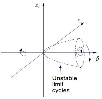
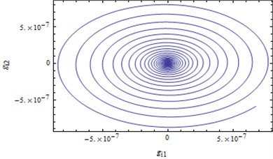
Evaluating (43) on the initial equilibrium $r_{1} = 0$ yields $\frac{d}{d r} (\frac{d r}{d τ^{'}}) = –1.46953 δ$ . The initial equilibrium is stable when $δ > 0$ and unstable when $δ < 0$ . In the same way, evaluating (43) on Hopf bifurcation solution (42) yields $\frac{d}{d r} (\frac{d r}{d τ^{'}}) = 5.72438 δ$ . So Hopf bifurcation solution (43) is unstable when $δ > 0$ and no meaning when $δ < 0$ . The bifurcation path is shown in Fig. 2. Fig. 3 displays unsteady Hopf bifurcation solution. From the above situations and Eq. (42), we can conclude that when $δ > 0$ the stable region of system (25) to (28) is very small, and system response is easy to diverge. Therefore the original blade-absorber system is also extremely sensitive, and this is a very dangerous situation in engineering.

Fig. 2Bifurcation path

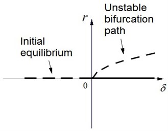
Fig. 3Unstable Hopf bifurcation solution

Now different values of parameter $δ$ are chosen to confirm the previous analytical results. Fourth-order Runge-Kutta method is adopted to simulate the response of Equations (25)-(28). Since this study focuses on local dynamic behaviors in the vicinity of critical point, the parameter $δ$ should be chosen near the critical point $δ =$ 0.

If the parameter is chosen as $δ = 0.001$ , a numerical solution starting from the initial point $(g_{r 1}, g_{i 1}, g_{r 2}, g_{i 2}) = (0.01,0.01,0.01,0.01)$ converges to the initial equilibrium solution, i.e. initial equilibrium solution is stable. It is indicative that system (25)-(28) disturbed by a small perturbation can still return its original state, which is shown in Fig. 4. Choosing the parameter as $δ = –0.001$ and starting from $(g_{r 1}, g_{i 1}, g_{r 2}, g_{i 2}) = (0.1,0.01,0.01,0),$ system response is divergence. It is indicative that system will produce large amplitude vibration, thereby causing damage to the whole structure. The numerical results are in good agreement with the theoretical analysis.

Fig. 4Trajectory projections converge to the initial equilibrium solution when δ=0.001

a)

b)

4.2. The case of double zero eigenvalues

Taking parameters as follows:

44

e = 0.05, ω_{β_{1}} = 1.75518, ω_{β_{2}} = 0.1, η_{1} = η_{2} = 0.01, γ = 0.15, d_{1} = 1,

e_{1} = 5, d_{2} = 0.001, e_{2} = 0.001, l_{1} = 0.01, l_{2} = 0.02, ω_{β_{1}} = 2, σ = σ_{0} = 0.1,

y_{0} = 0.597817 .

Jacobi matrix (29) has the eigenvalues $λ_{1,2} = 0$ , $λ_{3,4} = –0.16099±1.36954 i$ . We consider parameters $ω_{β_{1}}$ and $y_{0}$ perturbation parameters and use the parameter transformation $ω_{β_{1}} = 1.75518 + δ_{1}$ , $y_{0} = 0.597817 + δ_{2}$ . Then characteristic polynomial of the Jacobi matrix (29) becomes:

45

\tilde{f} (λ) = λ^{4} + {\tilde{R}}_{1} λ^{3} + {\tilde{R}}_{2} λ^{2} + {\tilde{R}}_{3} λ + {\tilde{R}}_{4},

where the specific forms of ${\tilde{R}}_{i}$ $(i = 1, 2, 3, 4)$ are too complex then omitted.

By Hurwitz criterion, the stability conditions for the initial equilibrium solution $(g_{r 1}, g_{i 1}, g_{r 2}, g_{i 2}) = (0,0, 0,0)$ are:

46

Δ_{1} = {\tilde{R}}_{1} > 0, Δ_{2} = {\tilde{R}}_{1} {\tilde{R}}_{2} - {\tilde{R}}_{3} > 0, Δ_{3} = {\tilde{R}}_{1} {\tilde{R}}_{2} - {\tilde{R}}_{3} > 0, Δ_{4} = {\tilde{R}}_{4} > 0 .

From the four inequalities above, we get the following four transition curves:

47

L_{1} : {\tilde{R}}_{1} = 0, L_{2} : {\tilde{R}}_{1} {\tilde{R}}_{2} - {\tilde{R}}_{3} = 0, L_{3} : {\tilde{R}}_{1} {\tilde{R}}_{2} - {\tilde{R}}_{3} = 0, L_{4} : {\tilde{R}}_{4} = 0 .

Since system local property near $(δ_{1}, δ_{2}) = (0,0)$ is only considered, $L_{4} > 0$ always holds in this region. Therefore when $L_{i} > 0$ $(i = 1, 2, 3)$ , initial equilibrium solution is stable, otherwise it is unstable. The transition curves in the vicinity of $(δ_{1}, δ_{2}) = (0,0)$ and stable region (shaded part) for initial equilibrium solution (E.S.) are shown in Fig. 5.

Fig. 5Transition curves and stable region in the case of double zero eigenvalue

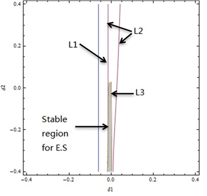
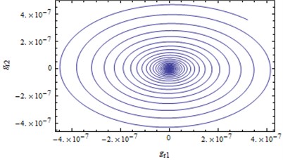
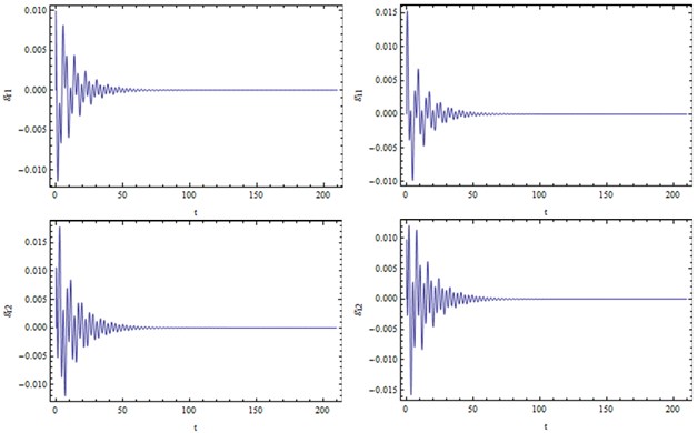
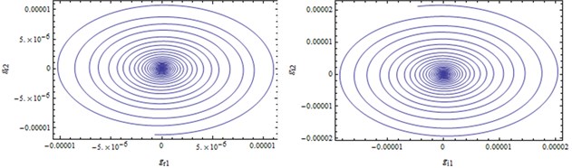
Fig. 6a) gr1, gi1, gr2, gi2 response process and b) phase diagrams of convergence to the origin

a)

b)

Now we will confirm the previous analysis by fourth-order Runge-Kutta method. Choosing parameter values of $δ_{1}$ and $δ_{2}$ from the stable region for E.S., such as $(δ_{1}, δ_{2}) = (–0.001, 0.01)$ , a numerical solution starting from an initial point $(g_{r 1}, g_{i 1}, g_{r 2}, g_{i 2}) = (0. 01, 0.01, 0.01, 0.01)$ converges to the origin, implying that the E.S. is stable. $g_{r 1}$ , $g_{i 1}$ , $g_{r 2}$ , $g_{i 2}$ response process as well as phase diagram projection on the $g_{r 1} - g_{r 2}$ and $g_{i 1} - g_{i 2}$ sub-spaces are shown in Fig. 6.

5. Conclusions

In this work, the dynamic behaviors of a helicopter blade-absorber model have been studied in detail. The research shows that helicopter blade-absorber vibration system has relatively rich in dynamic behaviors, and its dynamic analysis is of great necessity. When the stable conditions for the initial equilibrium solution of the bifurcation response equations are not satisfied, two kinds of critical points (characterized by a pair of purely imaginary eigenvalues and double zero eigenvalues) have been considered. Bifurcation path, transition curves and stable region have been obtained. All analytical predictions are agree with numerical results calculated by Runge-Kutta method. Note that in the blade-absorber system vibration process, the appearance of unstable Hopf solution is extremely dangerous, we should apply a bifurcation control or avoid taking system parameter in the vicinity of bifurcation point. Therefore, in order to achieve the purpose of absorbing vibration, ensure system safety, when designing system parameter, we must fully consider external excitation frequency, avoid the possible resonance region, and retain a certain safety margin.

References

Yu P. Analysis on double Hopf bifurcation using computer algebra with the aid of multiple scales. Nonlinear Dyn., Vol. 27, 2002, p. 19-53.

Search CrossRef
Bi Q., Yu P. Symbolic computation of normal forms for semi-simple cases. Journal of Comput. and Appl. Math., Vol. 102, 1999, p. 195-220.

Search CrossRef
Yu P. Computation of norm forms via a perturbation technique. Journal of Sound and Vibration, Vol. 211, 1998, p. 19-38.

Search CrossRef
Yu P. Symbolic computation of normal forms for resonant double Hopf bifurcations using a perturbation technique. Journal of Sound and Vibration, Vol. 247, 2001, p. 615-632.

Search CrossRef
Yu P., Yuan Y. The simplest normal form for the singularity of a pure imaginary pair and a zero eigenvalue. Dynamics of Continuous, Discrete and Impulsive Systems Series B, Application & Algorithms, Vol. 8, Issue 2, 2001, p. 219-249.

Search CrossRef
Yu P., Zhu S. Computation of the normal forms for general M-DOF systems using multiple time scales. Part I: Autonomous systems. Commun Nonlinear Sci Numer Simulat, Vol. 10, Issue 8, 2005, p. 869-905.

Search CrossRef
Zhu S., Yu P. Computation of the normal forms for general M-DOF systems using multiple time scales. Part II: Non-autonomous systems. Commun Nonlinear Sci Numer Simulat, Vol. 11, Issue 1, 2006, p. 45-81.

Search CrossRef
Han M., Yang J., Yu P. Hopf bifurcations for near-Hamiltonian systems. J. Bifurcation & Chaos, Vol. 19, Issue 12, 2009, p. 4117-4130.

Search CrossRef
Zhang X. H. Local bifurcations of nonlinear viscoelastic panel in supersonic flow. Commun Nonlinear Sci Numer Simulat, Vol. 18, 2013, p. 1931-1938.

Search CrossRef
Zhang X. H., Chen F. Q., Zhang H. L. Stability and local bifurcation of functionally graded material plate under transversal and in-plane excitations. Applied Mathematical Modelling, Vol. 37, Issue 10-11, 2013, p. 6639-6651.

Search CrossRef
Zhou L. Q., Chen F. Q. Stability and bifurcation analysis for a model of a nonlinear coupled pitch-roll ship. Mathematics and Computers in Simulation, Vol. 79, 2008, p. 149-166.

Search CrossRef
Wang X., Chen F. Q., Zhou L. Q. Stabilities and bifurcation for a flexible beam under a large linear motion with a combination parametric resonance. Nonlinear Dynamics, Vol. 56, 2009, p. 101-119.

Search CrossRef
Sang J. X. Study on dynamic stability and bifurcation of helicopters. Nanjing University of Aeronautics and Astronautics, 1995, (in Chinese).

Search CrossRef
Bramwell A. R. S., Done G., Balmford D. Bramwell’s helicopter dynamics. Second edition, Butterworth-Heinenmann, 2001.

Search CrossRef
Lee C. T., Shaw S. W. The non-linear dynamic response of paired centrifugal pendulum vibration absorbers. Journal of Sound and Vibration, Vol. 203, Issue 5, 1997, p. 731-743.

Search CrossRef
Chao C. P., Lee C. T., Shaw S. W. Non-union dynamics of multiple centrifugal pendulum vibration absorbers. Journal of Sound and Vibration, Vol. 204, Issue 6, 1997, p. 769-794.

Search CrossRef
Nester T. M. Experimental investigation of circular centrifugal pendulum vibration absorbers. Michigan State University, Master’s Thesis, 2002.

Search CrossRef
Miao W., Mouzakis T. Bifilar analysis study. NASA Contractor Report, NASA CR-159227, Vol. 1, 1980.

Search CrossRef
Cassarino S. J., Mouzakis T. Bifilar analysis user’s manual. NASA Contractor Report, NASA CR-159228, Vol. 2, 1980.8.

Search CrossRef
Taylor R. B., Teare P. A. Helicopter vibration reduction with pendulum absorbers. Journal of AHS, Vol. 20, Issue 3, 1975, p. 9-17.

Search CrossRef
Nagasaka I., Ishida Y., Koyama Y. Vibration suppression of a helicopter blades by pendulum absorbers. Transactions of the Japan Society of Mechanical Engineers, Vol. 73, 2007, p. 129-137.

Search CrossRef
Nagasaka I., Ishida Y., Koyama T. Vibration suppression of a helicopter fuselage by pendulum absorbers: rigid-body blades with aerodynamic excitation force. Journal of system design and dynamics, Vol. 2, 2008, p. 1230-1238.

Search CrossRef

About this article

Received

31 October 2013

Accepted

12 December 2013

Published

31 March 2014

Keywords

nonlinear coupled blade-absorber model

local bifurcation

stability

normal form

Acknowledgements

This paper is supported by Specialized Research Fund for the Doctoral Program of Higher Education of China (No. 20113218110002) and a project funded by the Priority Academic Program Development of Jiangsu Higher Education Institutions of China.

This is an open access article distributed under the Creative Commons Attribution License, which permits unrestricted use, distribution, and reproduction in any medium, provided the original work is properly cited.