Abstract
Piezoelectric ceramic exciter (PCE) have been used to experimentally study on the inherent and damping characteristics of thin-walled structures. However, due to its unknown excitation force level, it can not be applied on more practical cases in which accurate test of dynamic response is urgently needed. This research combines theory with experiment to calibrate sinusoidal excitation force generated by PCE. Firstly, a feedback attenuator was developed to help data acquisition instrument securely capture high-voltage excitation signal applied on PCE by high-voltage piezoelectric amplifier; Secondly, experimental research was conducted using a PCE, of type P-885.10 produced by PI in Germany, as object based on the PCE excitation feedback system to experimentally analyze its major influences on linear excitation capability, consequently a linear excitation equation was proposed to better regulate PCE to produce linear sinusoidal excitation signal; thirdly, a calibration method was proposed to exactly determine the level of sinusoidal excitation force of PCE based on the dynamics model of the cantilever beam excited by PCE, and its calibration principle and calibration process was explained in details. Finally, practicability and effectiveness of this calibration method was demonstrated by a calibration case. The results showed that if both of output signal voltage and excitation frequency meet the linear excitation equation, the concerned sinusoidal excitation force of PCE has a linear relationship with output signal voltage.
1. Introduction
Sinusoidal excitation is one of the common vibration excitation forms in the engineering field, which can be found in rotation, pulsation, oscillation and other vibration forms generated inevitably by driving ships, aeroplanes, vehicles, spacecrafts and etc. [1-2]. Sinusoidal excitation method (SEM) is one of the widely used excitation method for experimental study on vibration characteristics of mechanical structures [3-4]. It has many advantages compared to random excitation and transient excitation methods. Firstly, its vibration control algorithm is easy to develop while the control effect is better than others [5]. Secondly, its digital-signal processing procedures, i.e. integration, windowing and filtering is compact and fast-moving, which assist in our understanding of amplitude, phase, frequency and other information directly and visually [6]. At last, it also contributes to fault diagnosis and discovery of some nonlinear phenomena [7]. Therefore, SEM is frequently used in the following tests: (I) Vibration fatigue test. Impose a certain level of excitation energy to the test structure at its resonant frequency to objectively evaluate its fatigue resistance capability or fatigue properties with or without some damping coating [8]. (II) Predetermined frequency test. This method is often used to get the vibration level at concerned frequencies as well as to assess its anti-vibration capability. (III) Normal modal test. This method may assist in concentrating excitation energy on the single-frequency and thus getting modal shapes accurately [9].
Piezoelectric ceramic exciter (PCE) is a new type of micro-displacement device, which is usually be made in stacked structures in order to increase excitation energy [10]. It has some advantages like small volume, more reliable, high stiffness, high resolution, high frequency response and etc. PCE has been widely applied in micromachining, optics, electronics, aerospace, ultrasound and other fields [11-12]. Under the effect of an external electric field, PCE is equivalent to a parallel-plate capacitor which can be regarded as a capacitive load for its high-voltage piezoelectric amplifier (HPEA) [13-14]. According to the inverse piezoelectric effect, piezoelectric ceramic deforms in its polarization direction and generate vibration energy resulting from an applied electrical field. Therefore, it can be made into PCE with different sizes and shapes based on the required dynamic displacement responses.
During the past several years, increased attentions have been paid to the vibration application of PCE on thin-walled structures, such as blades, drum in the aerocraft engine and compressor, and metal sheet in automobile, helicopter and plane, and thin cylindrical shell and tube in the submarine and ship. Extensive works have been done in the area of experimental study on the inherent and damping characteristics of thin-walled structures. For example, Rongong and Tomlinson [15] employed PCE to randomly excite a ring with constrained layer damping by applying a band limited random signal, subsequently to estimate loss factors for each mode from the Nyquist circle to minimize the residual effects of close modes. Ivancic and Palazotto [16] employed PCE as excitation source to determined resonance frequencies and damping ratios of a titanium plate coated with magnesium aluminate spinel (mag spinel) through sine sweep test. Huang [17] pasted 12 PCEs on the first class compressor’s disk at different positions to provide for sufficient excitation energy and adopted laser holograph interference method to get a total of seven order mode shapes in the frequency range of 0-15000 Hz. However, there are some drawbacks in the application of PCE to excite thin-walled structures, because we do not exactly know its excitation force level, and thus we can not apply it on more practical cases in which accurate test of dynamic response is urgently needed. These limitations are serious obstacles to the development and advancement of structural modification, optimization design, response prediction and etc. Therefore, it is necessary to adopt certain calibration method to obtain sinusoidal excitation force of PCE to meet higher demands in accurate test and analysis of structural vibration.
Relevant experimental results show that PCE suffers from hysteresis, creep and other inherent nonlinear characteristics which usually lead to inconsistent behavior between the input voltage and output displacement [18-19]. And for better application of PCE, its nonlinear characteristics compensation technique and its dynamic response and control algorithm has drawn extensive research interest. Wang et al. [20] designed a controllable high voltage circuit to actuate PCE, and its static and dynamic characteristics are analyzed by experiments of sinusoidal and step response test, the results showed its amplitude of response will decrease with the increase of sinusoidal excitation frequency. Bonnail et al. [21] proposed a new procedure to characterize a PCE’s elongation at nanometer scale and established relationship between the excitation voltage and the tunneling current through the test data for indirect measurement of unknown elongation at different excitation voltage. Ben Mrad and Hu [22] presented a dynamic-hysteresis model of PCE, consequently the voltage-to-displacement dynamics were captured when sinusoidal-input voltage excitations were used at frequencies varying between 0.1 Hz and 800 Hz. Sung et al. [23] presented modeling and controller design method of PCE, obtained hysteretic behavior between input voltage and output displacement through the experiment, and designed a classical PID controller to regulate its output displacement.
Due to big differences among the following factors, such as PCE’s size, material property, load form of drive voltage supplied by HPEA and excitation frequency range, dynamic calibration of its sinusoidal excitation force have no rules to follow. One of the major difficulties is high-voltage excitation signal (10 V-200 V) applied on the PCE by high-voltage piezoelectric amplifier can hardly be simultaneously and securely captured by data acquisition instrument (DAI) whose secure voltage range is usually within 0 V-10 V; another one is that the commonly used dynamic calibration methods of the excitation force sensor, including impulse response, frequency response and step response methods and etc. [24-25], require lots of specialized equipments, which have the disadvantage of greater complexity and higher cost, so they are not well suitable for calibration excitation level of PCE. In order to solve these problems, further investigations are still needed, particularly, providing a simple while reliable way of determining its sinusoidal excitation force.
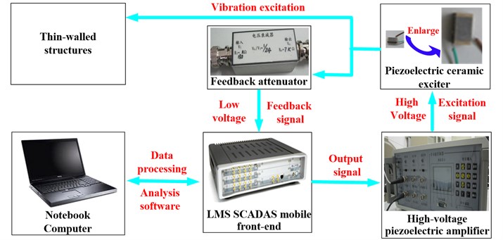
In this paper, a feedback attenuator was developed to adjust bias voltage to 0 V and convert high-voltage excitation signal into the low-voltage feedback signal. Which could help data acquisition instrument capture the real-time signal applied on the PCE by high-voltage piezoelectric amplifier and prevent data acquisition instrument being damaged when using it to directly collect high-voltage excitation signal. Section 2 was a brief introduction of PCE excitation feedback system based on this feedback attenuator as showed in Fig. 1, then went on to experimentally analyze major influences on PCE’s linear excitation capability in the course of normal use, and several conclusions were also drawn from results of experimental test. Thus, a linear excitation equation of PCE was proposed to better regulate PCE to produce linear sinusoidal excitation signal. In Section 3, a calibration method was proposed to exactly determine the level of sinusoidal excitation force of PCE based on the dynamics model of the cantilever beam excited by PCE, subsequently the key steps of the calibration method were explained in details. Finally in Section 4, practicability and effectiveness of this calibration method was demonstrated by a calibration case. The results showed that if both of output signal voltage and excitation frequency meet the linear excitation equation of PCE as proposed previously, the concerned sinusoidal excitation force of PCE has a linear relationship with output signal voltage.
Fig. 1Schematic of PCE excitation feedback system based on feedback attenuator
2. Experimental analysis on linear excitation capability of PCE
For calibrating sinusoidal excitation force of PCE, it is necessary to find out a way to evaluate its excitation capability firstly. In this section, PCE excitation feedback system was configurated to study its influencing factors experimentally. A linear excitation equation of PCE was proposed consequently, according to this equation, we can better regulate PCE to produce linear sinusoidal excitation signal, which could help solve concerned calibration problem.
2.1. PCE excitation feedback system
PCE excitation feedback system includes four main components, their detailed parameter and functions are:
1) PCE
A schematic of self-designed PCE excitation feedback system is shown in Fig. 1. The selected PCE’s item number is P-885.10 produced by PI in Germany, its dimensions is 5 mm×5 mm×9 mm, its capacitance is 0.6 μF with unipolar characteristics, weighs only 2 g. When it is being used, 2.5 V to 100 V bias voltage is needed to driver it to work in the positive voltage range securely, and it should be glued firmly on the measured specimen to make sure that its excitation force do not change gradually due to looseness of its contact area.
2) HPEA
High-voltage piezoelectric amplifier (Rhvd3c110v, made by RongZhiNaXin Corporation) is connected to data acquisition instrument (DAI) and is used to amplify low-voltage excitation signal from DAI to the higher level with a fixed gain (24 times magnification), and to provide stable bias voltage for PCE from 25 V to 110 V. Its voltage output resolution is 5 mV, the maximum output power is 100 W, the communication rate is 9600 Bps and the amount of output voltage can be displayed in real time by LCD screen.
3) Feedback attenuator
Feedback attenuator (jointly developed by the author’s research group and NanJingHongBin Corporation) is used to adjust bias voltage to 0 V and convert high-voltage excitation signal (10 V-200 V) applied on the PCE by HPEA into the low-voltage feedback signal (0 V-10 V) with a fixed attenuating ratio (correspond with HPEA’s magnification). It has two BNC ports, one is contacted to PEC’s two pins to receive high-voltage signal, and the other one is contacted to DAI to provide feedback signal which can be monitored and recorded by DAI simultaneously.
4) DAI and computer
LMS SCADAS Mobile Front-End is used to record excitation voltage signal of PCE through feedback attenuator and other response signals acquired by vibration sensors with 102.4 kHz sample rate within 1 mV-10 V input range (with16-channel data acquisition module) as well as to generate sinusoidal excitation signals (with 2-channel source module). It can also output sweep, random, chirp and other excitation signals with 24-bit resolution. LMS Test.Lab software, version 10 B, is used to control the data acquisition and generation. Besides, Dell notebook computer (with Intel Core i7 2.93 GHz processor and 4 G RAM) is used to operate LMS Test.Lab 10 B software and store measured data.
2.2. Influences on linear excitation capability of PCE
Some major factors which influence linear excitation capability of PCE are listed, such as excitation frequency, excitation voltage and bias voltage. Still, other factors like PCE’s size, material, capacitance, output power and magnification of HPEA and other hardware parameters undoubtedly affect PCE’s excitation performance. However, they appear to be particularly reliant on their relevant hardware performance that have been determined by manufacturers, rather than users or researchers, so we limit our discussion about linear excitation capability of PCE to the cases of practical application in this research.
2.2.1. A linearity criteria of sinusoidal excitation
Good practice in our test series dictates that sinusoidal excitation signal of PCE will be included in some harmonic frequencies resulting from these above influences, so it is necessary to propose a linearity criteria to regulate its harmonic frequency amplitude so as to reduce the nonlinear effects to the minimum. Conducting a fast Fourier transform (FFT) to convert the test data of excitation voltage signal through feedback attenuator to the frequency domain and obtain the amplitude of each harmonic frequency. Assuming that relationship between each harmonic frequency and base-frequency amplitude can meet Eq. (1), then we consider it has a good capability of linear excitation:
where, the subscript denotes the th harmonic frequency, is the linearity criteria, and is amplitude of base frequency and -harmonic frequency respectively, expressed in V.
2.2.2. Influence of bias voltage
In order to exclude the interference of other factors, PCE was clamped by a tweezers instead of being glued on the measured structure. First, set output signal voltage as 1 V and signal type as “sine” in the software, and defined its frequencies as 300 Hz and 3000 Hz; then, adjusted bias voltage at 25 V, 50 V and 75 V respectively in the HPEA and obtained excitation voltage amplitude of harmonic frequency and base-frequency by picking up each peak value in the spectrum which can be obtained by FFT through the test data of excitation voltage signal. Each amplitude result was averaged from the two test results, as listed in Table 1, and corresponding linearity criterion was calculated and also listed in Table 1. It can be observed that excitation voltage amplitude under different bias voltage is very close to each other, so linear excitation capability of PCE is little dependent on bias voltage applied on the PCE by HPEA.
Table 1Excitation voltage amplitude and linearity criteria under different bias voltage
Excitation frequency (Hz) | Bias voltage (V) | Excitation voltage amplitude (V) | Linear criterion | Linear criterion | ||
300 | 25 | 0.98 | 0 | 0 | 0 | 0 |
300 | 50 | 0.98 | 0 | 0 | 0 | 0 |
300 | 75 | 0.98 | 0 | 0 | 0 | 0 |
3000 | 25 | 0.90 | 0.031 | 0.03 | 0.03 | 0.03 |
3000 | 50 | 0.89 | 0.03 | 0.029 | 0.03 | 0.03 |
3000 | 75 | 0.90 | 0.03 | 0.03 | 0.03 | 0.03 |
2.2.3. Influence of excitation frequency
Fixed bias voltage at 75 V, set output signal voltage as 1 V and changed excitation frequency from 300 Hz to 6500 Hz in the software, experimental amplitudes and corresponding linearity criterion were obtained and listed in Table 2. Excitation voltage signal of PCE in time and frequency domain under 300 Hz and 4000 Hz were shown in Fig. 2 and Fig. 3. From which we can find out that excitation frequency has strong effect on linear excitation capability of PCE. When it is below 2800 Hz, base-frequency amplitude is dominant in the spectrum, where linear criterion 0.01 and 0.01, and thus excitation voltage signal is or close to linear. However, its harmonic amplitudes gradually raise with the rise of excitation frequency, i.e., 2-harmonic and 3-harmonic amplitudes are getting increasingly higher when excitation frequency is above 2800 Hz.
Fig. 2Excitation voltage signal in time and frequency domain at 300 Hz with 1 V output signal voltage
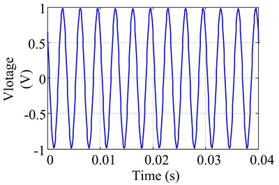
a) Excitation voltage signal in time domain
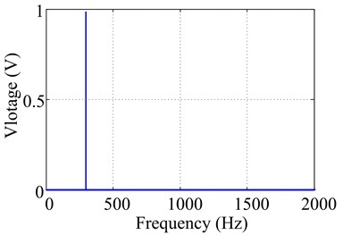
b) Spectrum of excitation voltage signal
Fig. 3Excitation voltage signal in time and frequency domain at 4000 Hz with 1 V output signal voltage
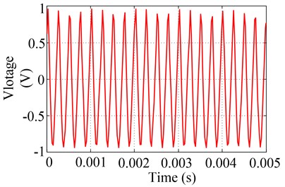
a) Excitation voltage signal in time domain
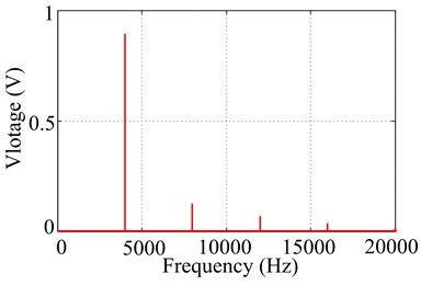
b) Spectrum of excitation voltage signal
Table 2Excitation voltage amplitude and linearity criteria at different excitation frequencies
Excitation frequency (Hz) | Output signal voltage (V) | Excitation voltage amplitude (V) | Linear criterion | Linear criterion | ||
300 | 1 | 0.98 | 0 | 0 | 0 | 0 |
600 | 1 | 0.98 | 0 | 0 | 0 | 0 |
900 | 1 | 0.97 | 0 | 0 | 0 | 0 |
1200 | 1 | 0.96 | 0 | 0 | 0 | 0 |
1500 | 1 | 0.95 | 0.003 | 0 | 0.003 | 0 |
1800 | 1 | 0.94 | 0.005 | 0 | 0.005 | 0 |
2100 | 1 | 0.93 | 0.006 | 0 | 0.006 | 0 |
2400 | 1 | 0.91 | 0.007 | 0 | 0.008 | 0 |
2700 | 1 | 0.9 | 0.008 | 0.003 | 0.009 | 0 |
2800 | 1 | 0.87 | 0.01 | 0.006 | 0.01 | 0.007 |
4300 | 1 | 0.86 | 0.15 | 0.06 | 0.17 | 0.070 |
5800 | 1 | 0.76 | 0.17 | 0.07 | 0.22 | 0.092 |
6500 | 1 | 0.71 | 0.18 | 0.08 | 0.25 | 0.113 |
2.2.4. Influence of output signal voltage
Still fixed bias voltage at 75 V, set output signal voltage as total 6 excitation levels in the software, namely 0.5 V, 1 V, 1.5 V, 2 V, 2.5 V, 3 V, and obtained experimental amplitudes of excitation voltage signal and corresponding linearity criterion at excitation frequency of 300 Hz and 2700 Hz respectively, as seen in Table 3 and Table 4. It can be observed that output signal voltage is also closely related to linear excitation capability of PCE. Once excitation frequency exceeds a certain critical value, harmonic amplitudes will gradually raise with the increase of output signal voltage.
Table 3Excitation voltage amplitude and linearity criteria under different output signal voltages at 300 Hz
Excitation frequency (Hz) | Output signal voltage (V) | Excitation voltage amplitude (V) | Linear criterion | Linear criterion | ||
300 | 0.5 | 0.49 | 0 | 0 | 0 | 0 |
300 | 1 | 0.98 | 0 | 0 | 0 | 0 |
300 | 1.5 | 1.48 | 0 | 0 | 0 | 0 |
300 | 2 | 1.97 | 0 | 0 | 0 | 0 |
300 | 2.5 | 2.46 | 0 | 0 | 0 | 0 |
300 | 3 | 2.95 | 0 | 0 | 0 | 0 |
Table 4Excitation voltage amplitude and linearity criteria under different output signal voltages at 2700 Hz
Excitation frequency (Hz) | Output signal voltage (V) | Excitation voltage amplitude (V) | Linear criterion | Linear criterion | ||
2700 | 0.5 | 0.45 | 0.003 | 0 | 0.007 | 0 |
2700 | 1 | 0.9 | 0.008 | 0.003 | 0.009 | 0.003 |
2700 | 1.5 | 1.27 | 0.23 | 0.09 | 0.18 | 0.07 |
2700 | 2 | 1.31 | 0.41 | 0.13 | 0.31 | 0.1 |
2700 | 2.5 | 1.2 | 0.46 | 0.19 | 0.38 | 0.16 |
2700 | 3 | 1.3 | 0.49 | 0.2 | 0.41 | 0.19 |
From the analysis of the above factors, it can be concluded that linear excitation capability of PCE is not dependent on excitation frequency or output signal voltage separately, but on both of them. In order to verify this conclusion, more detailed experimental test was conducted by adjusting excitation frequency and output signal voltage at different level. And test results were listed in Table 5, from which we can briefly summarize PCE’s characteristic as follows: it can be used as linear exciter with high output signal voltage, but only at lower excitation frequency. Each output signal voltage is related to a critical value of excitation frequency, named “critical frequency of linear excitation”, once excitation frequency exceeds this one, the spectrum of excitation voltage signal contains nonlinear harmonic amplitudes.
Table 5Excitation voltage amplitude and linearity criteria under different excitation frequencies and output signal voltages
Excitation frequency (Hz) | Output signal voltage (V) | Excitation voltage amplitude (V) | Linear criterion | Linear criterion | ||
300 | 1.5 | 1.47 | 0 | 0 | 0 | 0 |
900 | 1.5 | 1.46 | 0 | 0 | 0 | 0 |
1500 | 1.5 | 1.43 | 0 | 0 | 0 | 0 |
2000 | 1.5 | 1.38 | 0.008 | 0.004 | 0.006 | 0.003 |
2300 | 1.5 | 1.32 | 0.016 | 0.009 | 0.01 | 0.007 |
300 | 2 | 1.97 | 0 | 0 | 0 | 0 |
900 | 2 | 1.96 | 0 | 0 | 0 | 0 |
1200 | 2 | 1.95 | 0.01 | 0.01 | 0.005 | 0.005 |
1300 | 2 | 1.93 | 0.02 | 0.01 | 0.01 | 0.005 |
300 | 2.5 | 2.46 | 0 | 0 | 0 | 0 |
900 | 2.5 | 2.46 | 0.02 | 0.01 | 0.008 | 0.004 |
1000 | 2.5 | 2.44 | 0.03 | 0.02 | 0.01 | 0.008 |
300 | 3 | 2.95 | 0 | 0 | 0 | 0 |
600 | 3 | 2.93 | 0.03 | 0.02 | 0.01 | 0.007 |
2.3. Linear excitation equation
From the conclusion in Section 2.2, for objectively evaluating linear excitation capability of PCE, it should take into account the influences of excitation frequency and output signal voltage simultaneously (we will discuss how to convert output signal voltage into sinusoidal excitation force by some calibration method in Section 3). Since 2-harmonic frequency has higher effects on linear excitation than 3-harmonic frequency (), test data corresponding to 1 was chosen, as shown in Table 6, to establish linear excitation equation which could help us to better regulate PCE to produce linear sinusoidal excitation signal.
If linear evaluation index of PCE is introduced, the linear excitation equation may be characterized by Eq. (2):
where is a vector of critical frequencies of linear excitation, is a vector of output signal voltages. Additionally, is the fitting coefficient from experimental data.
Table 6Excitation frequency and voltage corresponding to S2≈ 1
Output signal voltage (V) | 0.5 | 1 | 1.5 | 2 | 2.5 | 3 |
Excitation voltage (V) | 0.48 | 0.87 | 1.32 | 1.93 | 2.44 | 2.93 |
Critical frequency of linear excitation (Hz) | 4000 | 2800 | 2300 | 1300 | 1000 | 600 |
It can be observed from Eq. (2) that when 1 V, the value of remains a fixed value no matter what the value of is. From this fact, we can deduce that:
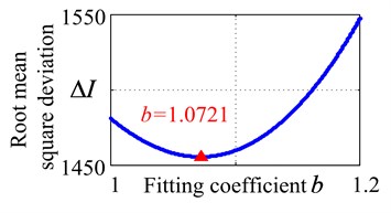
Based on experimental data from the Table 6, it can be known that should be larger than 1 to ensure the value of being a constant. Using least squares method we can determine the value of , which can be expressed as:
where, refers to the root mean square deviation.
Substitute Eq. (3) into the Eq. (4) and solving Eq. (4) by different fitting coefficient , until we finally get 1.072 at which is reach to its minimum, and the fitting coefficient/root mean square deviation relationship was showed in Fig. 4, whose horizontal and vertical axis is and , respectively.
Fig. 4The fitting coefficient/root mean square deviation relationship
2.4. Applications of the linear excitation equation
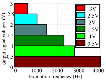
According to Eq. (2), PCE can be controlled effectively to produce sinusoidal excitation signal without nonlinear harmonic amplitudes. For example, if we want to use it to excite a structure or specimen at 1500 Hz, then we estimate the maximum output signal voltage should be below 2.06 V. Conversely, the critical frequency of linear excitation can also be acquired under the given output signal voltage. Moreover, we can further get its linear frequency-confidence interval, as seen in Fig. 5, by associating different output signal voltage with different colors, to evaluate its linear excitation capability.
Fig. 5Linear frequency-confidence interval of PCE
3. Calibration for sinusoidal excitation force of PCE
In this section, a method, for solving concerned calibration problem under the condition that PCE has already be effectively controlled by linear excitation equation in Section 2, is proposed. Since beam theory is quite mature and widely deployed and its inherent characteristics and vibration responses have a good agreement with experimental results [26]. Therefore, cantilever beam is the most common used model in both theoretical research and experimentally validation. We establish dynamics model of the cantilever beam excited by PCE as to stimulate the experimental process for exactly determining the level of sinusoidal excitation force.
3.1. Dynamics model of the cantilever beam subjected to sinusoidal excitation force of PCE
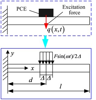
Experimental procedure of using PCE to excite the cantilever beam can be simulated by the following model, as shown in Fig. 6, here a classic Euler-Bernoulli beam with uniform cross-section is assumed and its bending vibration is of the major concern. -axis is presumed to locate in the centerline of beam and is the distance between clamp end and the geometric center of PCE, the length of the beam and PCE along the -axis is and respectively. Adopt distributed transverse loading, , acting on the differential segment of beam to simulate sinusoidal excitation force, its expression is shown as:
where refers to amplitude of sinusoidal excitation force in N, refers to angular excitation frequency in rad/s.
Fig. 6Dynamics model of the cantilever beam excited by PCE
Considering viscous damping, the bending vibrations of a uniform beam subjected to dynamic loading are described by the following equation:
where , , , are the Young’s modulus, second moment of area, mass per unit length, and transversedisplacement response. And and is damping coefficient of displacement velocity and deformation velocity respectively.
Introducing normal coordinates and solve the Eq. (6) by mode superposition method, we get displacement response of the cantilever beam as:
where represents vibration amplitude of -modal shape, represents the value of -modal coordinate.
In text books [26], that modal shape function, , of a cantilever beam is usually given by the following:
where represents excitation amplitude of vibration system related to amount of input energy, and represents a parameter associated with -natural frequency.
Introducing modal damping ratio and natural frequency (1.875, 4.694, 7.855, …, which is associated with mode shape) for the th mode and two constant coefficients, , , make the following assumptions:
Substitute Eq. (7), Eq. (9)-(11) into the Eq. (6), and according to the orthogonality conditions of any arbitrary shape, normalcoordinate response equation can be normalized as:
where is the generalized loading associated with mode shape , its expression is:
The Duhamel solution of Eq. (12) under zero initial conditions is:
where , is the natural frequency for the th mode with damping.
Dynamic loading of PCE can be equivalent to the distributed loading on the differential segment of beam, bring it into the Eq. (13) yields:
Substitute Eq. (15) into the Eq. (14) and add Eq. (8), by using Eq. (7) we can get dynamic response at any point in cantilever beam subjected to sinusoidal excitation force of PCE.
3.2. Calibration principle based on the dynamics model of the cantilever beam
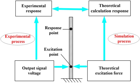
Schematic of calibration principle, as seen in Fig. 7, for determining the level of sinusoidal excitation force based on the dynamics model of the cantilever beam mainly involves three mapping: (I) Experimental process vs. simulation process; (II) Output signal voltages applied on the PCE by high-voltage piezoelectric amplifier vs. theoretical excitation force applied on dynamics model; (III) Response results of experiment vs. calculated results of dynamics model. On one hand, we carry out experimental test to get output signal voltages on the basis of PCE excitation feedback system and displacement response of cantilever beam specimen by Laser Doppler Vibrometer (its velocity response signal needs to be processed through the integral transform). On the other hand, at the same position of excitation and response signal, we use dynamics model of the cantilever beam proposed in Section 3.1 to calculate dynamic response subjected to some level of theoretical excitation force. When the calculated result of dynamics model have a good agreement with test result, i.e., its error is below 3 %, we regard this level of theoretical excitation force is equal to actual sinusoidal excitation force produced by PCE, and thus we successfully solve concerned calibration problem.
Fig. 7Calibration principle of sinusoidal excitation force of PCE based on the dynamics model of the cantilever beam
3.3. Calibration process
To obtain sinusoidal excitation force of PCE, nature frequencies, modal damping ratios and displacement responses of cantilever beam specimen are needed to be measured precisely as to update the dynamics model. The calibration process can be summed up as following:
1) Set up calibration system of sinusoidal excitation force of PCE.
There are three basic steps to set up calibration system of sinusoidal excitation force of PCE based on beam theory. The first is that using a torque wrench to hold beam specimen tightly in the clamping fixture to ensure the beam is in clamped-free boundary conditions. The second is choosing Laser Doppler Vibrometer to reveal displacement response at the top position of beam without contact. The third is setting up PCE excitation feedback system to record excitation voltage signal of PCE through feedback attenuator and response signal from Laser Doppler Vibrometer. To reduce the influence resulting from added mass and stiffness of PCE, it needs to be placed closely to the clamped end of cantilever beam and glued firmly by super glue 502.
2) Measure natural frequencies of cantilever beam specimen.
Experimental Modal Test was used to obtain frequency response function (FRF) of cantilever beam specimen. Firstly, random vibration signal amplified by HPEA is employed to driven PCE, and then excite cantilever beam specimen to vibrate. Next, the digital filtering technology is adapted to drop down the impact of the test noise to obtained response signal. At last, estimate FRF by the recorded excitation and response signals, from which natural frequency can be determined through each resonant peak, besides, modal damping ratio can also be identified by the half-power bandwidth method which is calculated by measuring the bandwidth of the frequency curve (or approximately 3 dB) down from the resonant peak. In order to obtain the accurate results, several different test points can be chosen and the average is used as the final experimental results, for providing inherent as well as damping parameters of the real specimen for dynamics model.
3) Obtain displacement amplitude under different output signal voltages.
Select frequency range in which PCE often works and divide this range into a number of tested frequency point, and sine excitation experiments are performed on each of these frequencies. On one hand, get the spectrum of velocity response signal in the laser point and convert it to displacements through integration process, consequently identify displacement amplitude. On the other hand, mark and record output signal voltages corresponding to this displacement amplitude.
4) Establish dynamics model and update this model through measured data.
Testing the geometry and physical parameters of specimen is the basis for establishment of dynamics model. As important input parameters for dynamics model, length, width, thickness of the cantilever beam and positions of measuring points are acquired by vernier caliper or micrometer yet with test error; physical parameters is somewhat unclear due to thermal deformation of the cutting process, hence they all need to be modified slightly before being as final input data for dynamics model. According to the description in Section 3.1, establish dynamics model of the cantilever beam subjected to sinusoidal excitation force of PCE. Firstly, roughly calculate natural frequencies based on this model. Then, update dynamics model by modifying material and geometric parameters until errors between theoretical and experimental result for each order natural frequency is less than 5 %.
5) Calculate dynamic response amplitude and calibrate sinusoidal excitation force.
Calculating dynamic response and calibrate sinusoidal excitation force of PCE based on the updated dynamics model can be divided into two steps. First, put measured damping parameter from step (2) into this model so as to get more reliable response result, since vibration response of the structure is highly dependent on damping performance of each mode. Then, at the same position of excitation and response signal, using this model to calculate dynamic response amplitude subjected to certain level of theoretical excitation force. Adjusting this force to levels where calculated result is close to the test result (its error is below 3 %). Thus, this level of theoretical excitation force can be regarded as actual sinusoidal excitation force produced by PCE.
6) Draw calibration curve of PCE at certain excitation frequency.
Repeat steps (3) to (5), change output signal voltage to get a series of value of displacement amplitude, and map each of them with calculated result, in this way we can clearly establish the relationship between output signal voltage and sinusoidal excitation force from updated dynamics model. Besides, calibration curve as well as its mathematical expression can be obtained by least square fitting technique, and the more we get value of vibration response at certain excitation frequency, the more precise calibration curve we can obtain.
4. A calibration case
The following will use the proposed methods to exactly determine the level of sinusoidal excitation force of PCE and apply calibration curve of PCE on the response measurement.
4.1. Calibration system setup
According to the calibration process in Section 3.3, calibration system of sinusoidal excitation force of PCE was set up by adding cantilever beam specimen and Laser Doppler Vibrometer to the PCE excitation feedback system in Fig. 1. A Ti-6Al-4V beam for this study is 280 mm×20 mm×1.5 mm (Young’s modulus is 110.32 GPa, Poisson’s ratio is 0.31, and the density is 4420 kg/m3), the effective test area was 250 mm×20 mm×1.5 mm with 30 mm in clamped region. A two piece fixture was designed to sandwich the beam specimen and four bolts, two beyond both ends of the beam and two near its centerline, were adjusted to 40 Nm to provide enough clamping force. The selected PCE, of type P-885.10 produced by PI in Germany with dimensions 5 mm×5 mm×9 mm, was glued firmly on the centerline of beam with 7 mm above the clamped end. Laser Doppler Vibrometer (Polytec PDV-100) was used to reveal the frequency and vibration displacement of the beam. Because it was not configured to take displacement measurements, its velocity measurements were converted to displacements by dividing where represents excitation frequency, and the distance from laser point to beam’s free end is 5 mm. Other instruments, such as HPEA, feedback attenuator, DAI and computer, were already described in Section 2.1. It is necessary to note that each distance parameter was measured by vernier caliper for three times and the average was used as test result, tests of nature frequencies, modal damping ratios and displacement responses of cantilever beam specimen were run at room temperature.
4.2. Test procedures and calibration results
4.2.1. Compare of natural frequencies
Experimental Modal Test was done between 0-1400 Hz to determine natural frequencies of cantilever beam specimen base on the calibration system in Section 4.1. Random output signal was set to driven PCE, and then excite cantilever beam specimen to vibrate. Polytec PDV-100, mounted to a rigid support, was used to measure the beam velocity at a single point. LMS Test.Lab software took excitation voltage signal through feedback attenuator and the beam’s response signal and conducted FFT to convert the data to the frequency domain. The output is an amplitude of velocity versus frequency graph, that is FRF, where each peak represents a natural frequency and mode damping ratio was determined by the “half-power bandwidth” calculation. Because FRF is a function of response signal divided by the excitation signal, natural frequencies and modal damping ratios can be correctly identified without necessarily knowing the excitation force level. In this test, the first five natural frequencies and mode damping ratios were identified and listed in Table 7 and Table 8.
Table 7Natural frequencies of the beam obtained by theoretical calculation and experimental test / Hz
Modal order | 1 | 2 | 3 | 4 | 5 |
Experiment | 23.4 | 144.5 | 403.1 | 789.1 | 1295.2 |
Theory | 23.9 | 149.9 | 419.6 | 822.3 | 1359.2 |
Error (%) | 2.14 | 3.74 | 4.09 | 4.21 | 4.94 |
Table 8Damping ratios of the beam obtained by experimental test
Modal order | 1 | 2 | 3 | 4 | 5 |
Damping ratio (%) | 2.13 | 0.35 | 0.14 | 0.07 | 0.12 |
Established a dynamics model of the cantilever beam and repeatedly calculated its natural frequencies through slightly modifying material and geometric parameters, if a good correlation exited between the theoretical and experimental results, this updated dynamics model can be used as a benchmark for calculating dynamic response as stated previously in the Section 3.2. Natural frequencies results of updated dynamics model were also listed in Table 6, it can be found out that the error is within an acceptable range (the theoretical calculation is less than 5 % of the experimental results for the first five modes). Therefore, this model closely approximates reality and can be used to calculate the vibration response of the cantilever beam.
4.2.2. Compare of dynamic response
After updated dynamics model of cantilever beam specimen was obtained, we can further compare theoretical calculation response with experimental results. For example, if sinusoidal excitation force at 300 Hz was mainly concerned, we needed to know the amplitude of dynamic response under this excitation level. On one hand, set output signal voltage in the LMS Test.Lab software as total 6 excitation levels, namely 0.5 V, 1 V, 1.5 V, 2 V, 2.5 V, 3 V, and defined signal type as “sine” to drive PCE to provide cantilever beam specimen with sinusoidal excitation energy (from linear frequency-confidence interval of PCE, as seen in Fig. 5, we already known that these voltage could not bring too large nonlinear harmonic amplitudes with 0.01 or 0.01). Then, obtained velocity response signal in the laser point under each output signal voltage and conducted FFT to get the spectrum of velocity response signal (expressed in the linear form due to its convenience to read peak value). Next, converted it to displacements through integration process and obtained the desired displacement amplitude by reading the peak value in the spectrum. In this way, we can also get displacement amplitudes under different output signal voltages at 300 Hz, and the experimental results were listed in the Table 9. It can be seen that dynamic response of cantilever beam specimen is less than 1 um, which is relatively small compared to engineering vibration level (usually large than 0.1 mm). However, Laser Doppler Vibrometer can still qualified for this micro-vibration test, because its displacement resolution can achieve to nanometer scale.
On the other hand, calculated dynamic response amplitude and calibrated sinusoidal excitation force. First, put measured damping ratios into the dynamics model, as seen in Table 8, and calculated displacement response amplitude at the same position with experiment. Then, repeatedly adjusted the level of theoretical excitation force until calculated displacement amplitude, as listed in Table 9, was close to the test result. It can be observed that mapping errors of dynamic response are within 3 %, so the calculated displacement amplitudes is trustworthy. Therefore, we can regard this level of theoretical excitation force as actual sinusoidal excitation force produced by PCE.
Table 9Calibration results of sinusoidal excitation force of PCE under different excitation voltage at 300 Hz
Experiment | Excitation voltage (V) | 0.5 | 1 | 1.5 | 2 | 2.5 | 3 |
Displacement amplitude (um) | 0.25 | 0.33 | 0.40 | 0.49 | 0.64 | 0.74 | |
Theory | Theoretical excitation force (N) | 0.11 | 0.14 | 0.17 | 0.21 | 0.28 | 0.32 |
Displacement amplitude (um) | 0.26 | 0.32 | 0.4 | 0.49 | 0.64 | 0.75 | |
Mapping error (%) | 1.05 | –1.44 | 0.19 | –0.36 | 0.31 | 0.69 | |
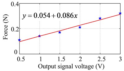
4.2.3. Draw calibration curve
According to theoretical and experimental data in Table 8, we can draw force/output signal voltage calibration curve at 300 Hz and thus we successfully determined the level of sinusoidal excitation force of PCE under this excitation frequency, as showed in Fig. 8, whose horizontal and vertical axis was output signal voltage and sinusoidal excitation force respectively. As it is clear from the plots, the excitation force raises when the output signal voltage increases. Besides, using least square fitting technique, we can further obtain its mathematical expression, , where represents output signal voltage and represents target force, it is obvious these two variables have a linear relationship. It should be noted that this calibration curve is based the calibration system as well as related hardware devices designed and configurated by the author’s research group, and different hardware devices are likely to cause different calibration results of sinusoidal excitation force of PCE at different frequencies. However, this calibration method can still be an important reference for solving similar calibration problems.
Fig. 8The calibration curve of sinusoidal excitation force of PCE at 300 Hz
4.3. The application of calibration curve of PCE
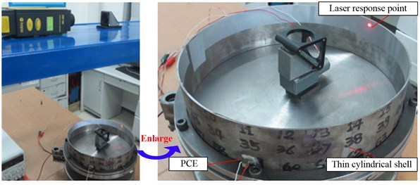
Repeated the above steps, calibration curves of PCE at other interested frequencies can be obtained. Thus, excitation force level of PCE can be clearly determined, which is one of most important parameters in accurate test of dynamic response. Therefore, PCE, with lighter quality and higher excitation frequency compared to the electromagnetic exciter, not only can be applied in the test area of inherent and damping characteristics, but also in the test area of vibration response of thin cylindrical shell by Laser Doppler Vibrometer, as seen in Fig. 9. FRF measurement (velocity over drive voltage) had been measured between the laser response point and one single excitation point with PCE pasted there, chirp excitation was applied on the tested shell by PCE with the following parameters: 0-3000 Hz frequency range; 70 % chirp length; 0.15 Hz frequency resolution; 10 averages; uniform windows. By identifying FRF of thin cylindrical shell, as given in Fig. 10, the first order natural frequency was 300 Hz.
Fig. 9Photograph of the tested thin cylindrical shell being excited by PCE
Next, sine excitation experiment at 300 Hz was performed which was hope to excite cylindrical shell under first order resonance, excitation voltage signal of PCE at 300 Hz with 3 V output signal voltage was shown in Fig. 11 and response signal of thin cylindrical shell was shown in Fig. 12. Using the calibration curve in Fig. 8, we had known that the sinusoidal excitation force corresponding to 3 V voltage was about 0.32 N. Beside, we can acquire response level, about 0.0009 m/s (equal to 0.48 um), by identifying the peak of base frequency in the spectrum of response signal. It should be noted that some harmonic amplitudes was also observed in this case, the main reasons for this were: (1) For this PCE, of type P-885.10, its excitation force was a bit small, so it did not adequately excite the tested shell under resonance. Thus, response measurement was interfered by environmental noise. (2) Influences of experimental boundary condition or nonuniform thickness of the tested shell may lead to the rise of harmonic frequencies. Therefore, for obtaining desired response data, we needed to use larger PCE or adopt multi-point excitation technique with more PCEs to provide sufficient excitation energy for the tested shell; in the meantime, we should reduce the nonlinear effects of above influences.
Fig. 10FRF of the tested thin cylindrical shell
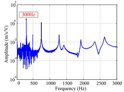
Fig. 11Excitation voltage signal in time and frequency domain at 300 Hz with 3 V output signal voltage
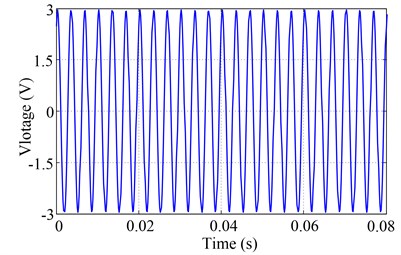
a) Excitation voltage signal in time domain
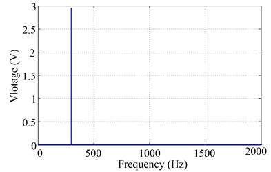
b) Spectrum of excitation voltage signal
Fig. 12Response signal of thin cylindrical shell in time and frequency domain
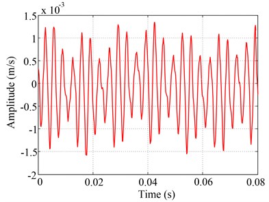
a) Response signal in time domain
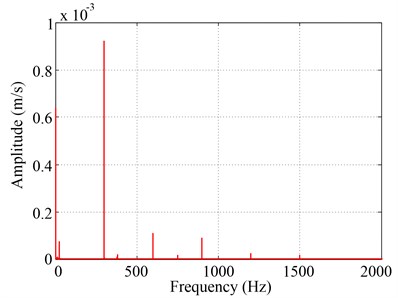
b) Spectrum of response signal
5. Conclusions
This research combines theory with experiment to exactly determine the level of sinusoidal excitation force generated by PCE. Based on the analysis and experimental results, the following conclusions can be drawn:
1) Linear excitation capability of PCE is little dependent on bias voltage applied by high-voltage piezoelectric amplifier, but closely related to output signal voltage and excitation frequency. The harmonic amplitudes of excitation voltage signal through feedback attenuator are getting increasingly higher with the rise of output signal voltage and excitation frequency. It is difficulty and impractical to accurately calibrate its sinusoidal excitation force in this condition.
2) PCE can still be used as linear exciter with higher excitation force, but only at lower excitation frequency. Each output signal voltage is related to a critical value of excitation frequency, called “critical frequency of linear excitation”, once excitation frequency exceeds this one, the spectrum of excitation voltage signal will contain nonlinear harmonic amplitudes.
3) PCE can be regulated effectively to produce sinusoidal excitation signal without nonlinear harmonic amplitudes by using linear excitation equation, which could help solve concerned calibration problem.
4) A calibration method, based on dynamics model of the cantilever beam, can be used to exactly determining the level of sinusoidal excitation force generated by PCE. And its key steps are as follow: (I) Set up calibration system; (II) Measure natural frequencies of cantilever beam specimen; (III) Obtain displacement amplitude under different output signal voltages; (IV) Establish dynamics model and update this model through measured data; (V) Calculate dynamic response amplitude and calibrate sinusoidal excitation force; (VI) Draw calibration curve of PCE at certain excitation frequency.
References
-
McConnell K. G., Varoto P. S. Vibration testing: theory and practice. Second Edition, John Wiley & Sons, Seoul, 1995.
-
Istvan L. V., Beranek L. L. Noise and vibration control engineering: principles and applications. New York, Wiley, 2006.
-
Link A., Täubner A., Wabinski W., et al. Modelling accelerometers for transient signals using calibration measurements upon sinusoidal excitation. Measurement, Vol. 40, Issue 9, 2007, p. 928-935.
-
Lee H. P. Stability of a cantilever beam with tip mass subject to axial sinusoidal excitations. Journal of Sound and Vibration, Vol. 183, Issue 1, 1995, p. 91-98.
-
Lin F. C., Yang S. M. Instantaneous shaft radial force control with sinusoidal excitations for switched reluctance motors. Energy Conversion, Vol. 22, Issue 3, 2007, p. 629-636.
-
Vizireanu D. N. A simple and precise real-time four point single sinusoid signals instantaneous frequency estimation method for portable DSP based instrumentation. Measurement, Vol. 44, Issue 2, 2011, p. 500-502.
-
Peng Z. K., Lang Z. Q. Detecting the position of non-linear component in periodic structures from the system responses to dual sinusoidal excitations. International Journal of Non-Linear Mechanics, Vol. 42, Issue 9, 2007, p. 1074-1083.
-
George T. J., Seidt J., Herman Shen M. H., et al. Development of a novel vibration-based fatigue testing methodology. International Journal of Fatigue, Vol. 26, Issue 5, 2004, p. 477-486.
-
Wright J. R., Cooper J. E., Desforges M. J. Normal-mode force appropriation-theory and application. Mechanical Systems and Signal Processing, Vol. 13, Issue 2, 1999, p. 217-240.
-
Adriaens H., De Koning W. L., Banning R. Modeling piezoelectric actuators. Mechatronics, Vol. 5, Issue 4, 2000, p. 331-341.
-
Chu X. C., Ma L., Li L. T. A disk – pivot structure micro piezoelectric actuator using vibration mode B11. Ultrasonics, Vol. 44, 2006, p. 561-564.
-
King T., Preston M., Murphy B., et al. Piezoelectric ceramic actuators: a review of machinery applications. Precision Engineering, Vol. 12, Issue 3, 1990, p. 131-136.
-
Karpelson M., Wei G. Y., Wood R. J. Driving high voltage piezoelectric actuators in microrobotic applications. Sensors and Actuators A, Physical, Vol. 176, 2012, p. 78-89.
-
Main J. A., Newton D. V., Massengill L., et al. Efficient power amplifiers for piezoelectric applications. Smart Materials and Structures, Vol. 5, Issue 6, 1996, p. 766-775.
-
Rongong J., Tomlinson G. Suppression of ring vibration modes of high nodal diameter using constrained layer damping methods. Smart Materials and Structures, Vol. 5, Issue 5, 1999, p. 672-684.
-
Ivancic F., Palazotto A. Experimental considerations for determining the damping coefficients of hard coatings. Journal of Aerospace Engineering, Vol. 18, Issue 1, 2005, p. 8-17.
-
Huang A. P. Test of vibration character and analysis of resonance speed character for disk. Measurement & Control Technology, Vol. 26, Issue 4, 2007, p. 14-15.
-
Ge P., Jouaneh M. Modeling hysteresis in piezoceramic actuators. Precision Engineering, Vol. 17, Issue 3, 1995, p. 211-221.
-
Jung H., Gweon D. G. Creep characteristics of piezoelectric actuators. Review of Scientific Instruments, Vol. 71, Issue 4, 2000, p. 1896-1900.
-
Wang X., Chu Y., Zhai Z. Research of micro-positioning system based on piezoelectric actuator. Electronic Measurement & Instruments, 9th International Conference on, 2009, p. 1-897-1-902.
-
Bonnail N., Tonneau D., Capolino G. A., et al. Dynamic and static responses of a piezoelectric actuator at nanometer scale elongations. Industry Applications Conference, 2000, p. 293-298.
-
Mrad R. B., Hu H. A model for voltage-to-displacement dynamics in piezoceramic actuators subject to dynamic-voltage excitations. Mechatronics, Vol. 7, Issue 4, 2002, p. 479-489.
-
Sung B. J., Lee E. W., Lee J. G. Dynamic modeling and displacement control of the piezoelectric actuator. Electrical Machines and Systems, 2007, p. 1902-1907.
-
Hou Y. L., Yao J. T., Zeng D. X., et al. Development and calibration of a hyperstatic six-component force/torque sensor. Chinese Journal of Mechanical Engineering, Vol. 22, Issue 4, 2009, p. 505-513.
-
Fujii Y. Toward dynamic force calibration. Measurement, Vol. 42, Issue 7, 2009, p. 1039-1044.
-
Sinha A. K. Vibration of mechanical systems. Cambridge University Press, London, 2010.
About this article
This study was supported by the National Natural Science Foundation of China, 51375079.
