Determination method of the structure size interval of dynamic similar models for predicting vibration characteristics of the isotropic sandwich plates

Luo, Zhong; Zhao, Xueyan; Zhu, Yunpeng; Li, Jianzhang

Journal of Vibroengineering

Browse Journal

Submit article

Published: 31 March 2014

Check for updates

Determination method of the structure size interval of dynamic similar models for predicting vibration characteristics of the isotropic sandwich plates

Zhong Luo¹

Xueyan Zhao²

Yunpeng Zhu³

Jianzhang Li⁴

^{1, 3, 4}School of Mechanical Engineering & Automation, Northeastern University, China

²Department of Automatic Control and Systems Engineering, University of Sheffield, UK

Corresponding Author:

Xueyan Zhao

Cite the article Download PDF

Downloads 1260

Abstract

A method is studied for determining the structure size interval of dynamic similar models of the isotropic sandwich plates. Firstly, a comparison between the two theories of plates, the Resineer theory and the Hoff theory, is conducted, including their governing equations and the ANSYS analytic solutions of frequency. The Resineer theory is chosen as the basic theory of this paper finally. Secondly, the scaling laws between the model and prototype of isotropic sandwich plate are established by combining the dimensional analysis and governing analysis. Both complete and incomplete geometric similarity conditions are discussed. Thirdly, the determination method of the structure size interval of the models is proposed. The nature vibration mode keeps the same and the nature frequency and harmonic response keep in proportion with the prototype of the sandwich plate. At last, the flow step of the intervals determination method is given.

1. Introduction

An isotropic sandwich plate typically consists of two stiff and strong thin face sheets, which are made of metallic or fiber composite material and a thick but low density core, which is between the two face sheets and bonds them together. Such sandwich construction has been widely used in modern engineering, especially in aeronautical, marine and other mechanical industries for decades since it offers the possibility of achieving high bending stiffness with little weight penalty. The investigation of the dynamic characteristics has become more and more important with the increasing use of sandwich constructions. Significant dynamic characteristic of the sandwich construction must be evaluated by experiments before it is applied in practical engineering. However, the experimental evaluation of sandwich plate is costly and time consuming. Consequently, a dynamic similarity scaled down model, which is much easier to work with, is used to predict the behavior of the prototype. Therefore, a reduction in cost and time can be achieved.

Scaling laws of sandwich plates have been studied extensively by many researchers. Morton [1] discussed the application of scaling laws to fiber isotropic laminates based on dimensional analysis, particularly emphasized the case of impact load, and it was shown that lay-up of laminates was important in assessing the likely validity of scale model tests. Stimitses and Rezaeepazhand [2-4] studied the scaling laws of incomplete geometric similarity models for predicting the laminate plate and shell buckling and free vibration. In their studies, scaling laws of different material properties, number of plies and geometric size were derived by using the governing equations of laminated plate and shell. Qian [5-6] used governing equations to establish the scaling laws of the impulse response of laminated plates, the results showed that analytical scaling rules could accurately describe the undamaged response to impact and when the plate dimensions, projectile dimensions and impact parameters all varied, the results were found to follow the scaling rules closely. Ungbhakorn and Singhatanadgid [7-8] established the scaling laws of anti-symmetric cross-ply and angle-ply isotropic laminated plates by applying the similitude transformation to governing equations of buckling and frequency directly, partial similitude was considered and the scaling laws which yield good agreement were recommended. Though the method which based on the direct use of the “governing equations” is more convenient than dimensional analysis, it is not so effective in predicting the dynamic response. In the study of Rosa and Franco [9], a structure similitude was proposed for the analysis of the dynamic response of plates or assemblies of plates. Similitude laws were defined by looking for equalities in the structural response, when the damping was modified, a mean response could be predicted in similitude. The structure responses for different fluid-structure interaction parameters were demonstrated for a variety of structure boundary conditions under water by Bachynski [10]. Yazdi [11] presented the establishment of the scaling laws for dynamic aeroelastic stability of laminated plates based on the direct use of governing equations. The results indicated that the models which had different parameters with those of the prototype could predict the flutter behavior of the prototype with good accuracy.

Some studies concerning the use of structure size intervals have been conducted in the past. Rezaeepazhand [12-13] presented to what extent similarity theory can be applied to in the design of a scaled down model. Since the intervals were given by experiments, the method finding the applicable structure size intervals was still not clear.

In this paper, intending to discuss the problem associated with the design of dynamic similar scale-down models in analyzing the dynamics characteristic of isotropic sandwich plates. A general determination method of the structure size interval of dynamic similar models of the isotropic sandwich plates was studied based on the Resineer theory of plates. The effectiveness of all these works is verified by numerical examples.

2. The comparative study of the theories of plates

The interested sandwich plate is shown in Figure 1. It consists of two face sheets with thicknesses $t_{h}$ , and length and width $b$ , $a$ and one core with thickness $h$ . The faces and the core are all isotropic with their principal directions along $x y z$ axes. The Reissner theory of plates and the Hoff theory of plates are two classical theories for analyzing the isotropic sandwich plates. Their assumptions and applicability are listed in Table 1.

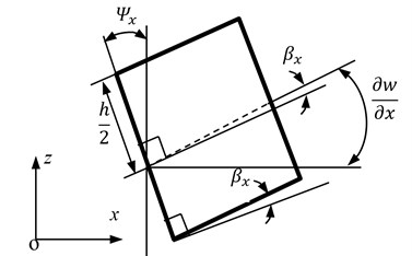
Table 1 shows that both the Renisser theory and the Hoff theory are able to analyze the dynamic characteristics of the isotropic sandwich plate. In the assumptions of the Hoff theory, the flexural stiffness $D_{f}$ of the isotropic sandwich plate’s face sheets is significant. In both the Renisser theory and the Hoff theory, the slope of the panel along the $x$ axis can be written as $\partial w / \partial x = ψ_{x} + β_{x}$ , where $ψ_{x}$ is the rotation of cross-section originally perpendicular to the $x$ axis and $β_{x}$ is the shear deformation (shown in Figure 2).

Table 1Two plates theories

Theory	Assumption	Applicability
Reissner	(1) The face sheets are thin compared to the core and in a state of plane stress ( $σ_{z} = τ_{x z} = τ_{y z} = 0$ ) (2) The in-plane stresses in the core are negligible ( $σ_{x} = σ_{y} = τ_{x y} = 0$ ) (3) The in-plane displacements in the core, $u$ and $v$ , are linear in the thickness coordinate, $z$ axis. (4) The out-of-plane displacement $w$ is independent of the $z$ coordinate, i.e. $ε_{z} = \frac{\partial w}{\partial z} = 0$	Critical load and low-order natural frequency of the isotropic sandwich plates
Hoff	(1) The face sheets are thin compared to the core but its flexural stiffness has to be considered. (2) The in-plane stresses in the core are negligible ( $σ_{x} = σ_{y} = τ_{x y} = 0$ ) (3) The in-plane displacements in the core, $u$ and $v$ , are linear in the thickness coordinate, $z$ axis (4) The out-of-plane displacement $w$ is independent of the $z$ coordinate, i.e. $ε_{z} = \frac{\partial w}{\partial z} = 0$	Concentrated load and high-order natural frequency of the isotropic sandwich plates

Fig. 1Structure of isotropic a sandwich plate

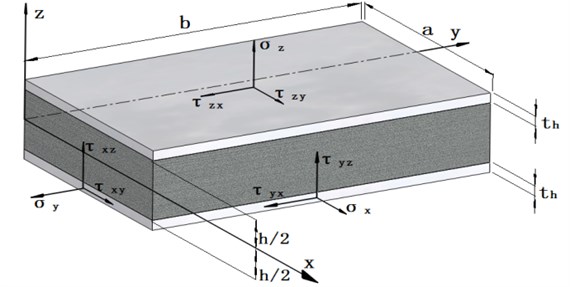
Fig. 2Deformation of core element in the x-z plane

2.1. Differences and relations of governing equations

In this paper, the isotropic sandwich plate in Figure 1 is considered to be rectangular, and the dimension condition is $a > b$ . The parameters of the isotropic sandwich plate are listed in Table 2.

Table 2Parameters of the isotropic sandwich plate

Parameter	Meaning	Parameter	Meaning
$D$	Flexural stiffness of isotropic sandwich plate	$ψ_{x}$	Rotation of $x$ coordinate
$μ_{f}$	Poisson’s ratio of face sheets	$ψ_{y}$	Rotation of $y$ coordinate
$E_{f}$	Young module of face sheets	$w$	Deflection
$K_{C}$	Shear stiffness of face sheets	$G_{c}$	Shear module of core
$a$	Length in $x$ coordinate	$b$	Length in $y$ coordinate

According to the Renisser theory, the governing equations of the isotropic sandwich plate can be written as [14]:

1

D (\frac{\partial^{2} ψ_{x}}{\partial x^{2}} + \frac{1}{2} (1 - μ_{f}) \frac{\partial^{2} ψ_{x}}{\partial y^{2}} + \frac{1}{2} (1 + μ_{f}) \frac{\partial^{2} ψ_{y}}{\partial x y}) + K_{C} (\frac{\partial w}{\partial x} - ψ_{x}) = 0,

2

D (\frac{1}{2} (1 - μ_{f}) \frac{\partial^{2} ψ_{y}}{\partial x^{2}} + \frac{\partial^{2} ψ_{y}}{\partial y^{2}} + \frac{1}{2} (1 + μ_{f}) \frac{\partial^{2} ψ_{x}}{\partial x y}) + K_{C} (\frac{\partial w}{\partial y} - ψ_{y}) = 0,

3

K_{C} (\frac{\partial^{2} w}{\partial x^{2}} + \frac{\partial^{2} w}{\partial y^{2}} - \frac{\partial ψ_{x}}{\partial x} - \frac{\partial ψ_{y}}{\partial y}) + N_{x} \frac{\partial^{2} w}{\partial x^{2}} + N_{y} \frac{\partial^{2} w}{\partial y^{2}} + N_{x y} \frac{\partial^{2} w}{\partial x y} + q = 0,

where, $D = \frac{E_{f} {(h + t_{h})}^{2} t}{2 (1 - {μ_{f}}^{2})}$ , $K_{C} = G_{c} (h + t_{h})$ , $N_{x}$ , $N_{y}$ , $N_{x y}$ denote the in-plane loads and $q$ denotes the external load.

The governing equations of the isotropic sandwich plate in the Hoff theory can be represented by the expressions:

4

D (\frac{\partial^{2} ψ_{x}}{\partial x^{2}} + \frac{1}{2} (1 - μ_{f}) \frac{\partial^{2} ψ_{x}}{\partial y^{2}} + \frac{1}{2} (1 + μ_{f}) \frac{\partial^{2} ψ_{y}}{\partial x y}) + K_{C} (\frac{\partial w}{\partial x} - ψ_{x}) = 0,

5

D (\frac{1}{2} (1 - μ_{f}) \frac{\partial^{2} ψ_{y}}{\partial x^{2}} + \frac{\partial^{2} ψ_{y}}{\partial y^{2}} + \frac{1}{2} (1 + μ_{f}) \frac{\partial^{2} ψ_{x}}{\partial x y}) + K_{C} (\frac{\partial w}{\partial y} - ψ_{y}) = 0,

6

K_{C} (\frac{\partial^{2} w}{\partial x^{2}} + \frac{\partial^{2} w}{\partial y^{2}} - \frac{\partial ψ_{x}}{\partial x} - \frac{\partial ψ_{y}}{\partial y}) - 2 D_{f} \nabla^{2} \nabla^{2} w + N_{x} \frac{\partial^{2} w}{\partial x^{2}} + N_{y} \frac{\partial^{2} w}{\partial y^{2}} + N_{x y} \frac{\partial^{2} w}{\partial x y} + q = 0,

where $\nabla^{2}$ is Laplace operator, $\nabla^{2} = \frac{\partial^{2}}{\partial x^{2}} + \frac{\partial^{2}}{\partial y^{2}}$ and $D_{f} = \frac{E_{f} {t_{h}}^{3}}{12 (1 - {μ_{f}}^{2})}$ .

It can be indicated obviously that Eq. (1) is the same as Eq. (4) and Eq. (2) is identical with Eq. (5). While Eq. (6) has one more term: $- 2 D_{f} \nabla^{2} \nabla^{2} w$ than Eq. (3), this is incurred by the face sheets’ flexural stiffness of the isotropic sandwich plate.

In Eq. (3) and Eq. (6), $w, ψ_{x}, ψ_{y}$ are unknown, so Hu Haichang [14] simplified the equations by replacing $w, ψ_{x}, ψ_{y}$ with two other functions $ω$ , $f$ and defined the transformation as follows:

7

ψ_{x} = \frac{\partial ω}{\partial x} + \frac{\partial f}{\partial y}, ψ_{y} = \frac{\partial ω}{\partial y} - \frac{\partial f}{\partial x} .

After the transformation, the governing equations are simplified as follows:

8

\frac{D}{2} (1 - μ_{f}) \nabla^{2} f - K_{C} f = 0,

9

D \nabla^{2} ω + K_{C} (w - ω) = 0 .

According to Eq. (9), the following relationship can be achieved:

10

w = ω - \frac{D}{K_{C}} \nabla^{2} ω .

$f \equiv 0$ is defined as the boundary condition of the simply supported plate [3], substitution of Eq. (7) and Eq. (10) into Eq. (6) results into the simplified equation of the Hoff theory:

11

(D + 2 D_{f}) \nabla^{2} \nabla^{2} ω - 2 \frac{D D_{f}}{K_{C}} \nabla^{2} \nabla^{2} \nabla^{2} ω = (N_{x} \frac{\partial^{2}}{\partial x^{2}} + N_{y} \frac{\partial^{2}}{\partial y^{2}} + N_{x y} \frac{\partial^{2}}{\partial x y}) (ω - \frac{D}{K_{C}} \nabla^{2} ω) + q .

According to Ref. [14], the simplified equation of the Renisser theory is:

12

D \nabla^{2} \nabla^{2} ω = (N_{x} \frac{\partial^{2}}{\partial x^{2}} + N_{y} \frac{\partial^{2}}{\partial y^{2}} + N_{x y} \frac{\partial^{2}}{\partial x y}) (ω - \frac{D}{K_{C}} \nabla^{2} ω) + q .

Eq. (11) has one more term $2 D_{f} \nabla^{2} \nabla^{2} (ω - \frac{D}{K_{C}} \nabla^{2} ω)$ than Eq. (12).

2.2. The comparison of analytic solution of natural frequency

It is assumed that the simply supported isotropic sandwich plate shown in Figure 1 is free of any transverse loads and in-plane normal and shear loads ( $N_{x} = N_{y} = N_{x y} = 0$ ) except the inertia force $q_{i}$ . The inertia force is $q_{i} = ρ \frac{\partial^{2} w}{\partial t^{2}}$ , where $ρ$ is the mass area ratio. In order to distinguish the function $ω$ , $\bar{ω}$ is used to denote natural frequency.

For the simply supported plate, the boundary conditions of the Hoff theory are:

13

x = 0, a :

\{\begin{array}{l} ω = 0, \\ \frac{\partial^{2} ω}{\partial x^{2}} = 0, \\ \frac{\partial f}{\partial x} = 0, \end{array}

14

y = 0, b :

\{\begin{array}{l} ω = 0, \\ \frac{\partial^{2} ω}{\partial y^{2}} = 0, \\ \frac{\partial f}{\partial y} = 0 . \end{array}

Due to $f \equiv 0$ , we get:

15

x = 0, a :

\{\begin{array}{l} ω = 0, \\ \frac{\partial^{2} ω}{\partial x^{2}} = 0, \end{array}

16

y = 0, b :

\{\begin{array}{l} ω = 0, \\ \frac{\partial^{2} ω}{\partial y^{2}} = 0 . \end{array}

Replace $ω$ by modal function $W (x, y)$ which satisfies the following boundary conditions:

17

ω = (A \cos \bar{ω} t + B \sin \bar{ω} t) W (x, y) .

If only the inertia force in Eq. (11) is considered, the free vibration characteristics are governed by:

18

(D + 2 D_{f}) \nabla^{2} \nabla^{2} ω - 2 \frac{D D_{f}}{K_{C}} \nabla^{2} \nabla^{2} \nabla^{2} ω = ρ \frac{\partial^{2}}{\partial t^{2}} (ω - \frac{D}{K_{C}} \nabla^{2} ω) .

Substitute Eq. (17) into Eq. (18), then:

19

(D + 2 D_{f}) \nabla^{2} \nabla^{2} W (x, y) - 2 \frac{D D_{f}}{K_{C}} \nabla^{2} \nabla^{2} \nabla^{2} W (x, y) = ρ {\bar{ω}}^{2} (W (x, y) - \frac{D}{K_{C}} \nabla^{2} W (x, y)) .

Substitute $W (x, y) = A_{m n} \sin \frac{m π x}{a} si n \frac{n π y}{b}$ into Eq. (19), then:

20

Ω = \frac{{(β^{2} m^{2} + n^{2})}^{2}}{1 + δ_{b} (β^{2} m^{2} + n^{2})} + k_{f} {(β^{2} m^{2} + n^{2})}^{2} = {(β^{2} m^{2} + n^{2})}^{2} [\frac{1}{1 + δ_{b} (β^{2} m^{2} + n^{2})} + k_{f}],

where $Ω = \frac{b^{4}}{π^{4}} \frac{ρ {\bar{ω}}^{2}}{D_{k}}$ , $β = \frac{b}{a}$ , $δ_{b} = \frac{π^{2} D}{b^{2} K_{C}}$ and $k_{f} = \frac{2 D_{f}}{D}$ .

When $k_{f}$ is neglected, Eq. (20) becomes:

21

Ω = \frac{{(β^{2} m^{2} + n^{2})}^{2}}{1 + δ_{b} (β^{2} m^{2} + n^{2})} .

Eq. (21) is the analytic solution of the natural frequency in the Renisser theory, which neglects the flexural stiffness of face sheets.

2.3. The choice of the plate theory

In this section, the applicable analytical method is chosen and verified by comparing the two theories’ analytic solutions of frequency with the ANSYS results. I SHELL91 element is applied in ANSYS modeling, and the model is meshed by quadrilateral meshes. Consider the following example:

It is assumed that the isotropic sandwich plate is with $a = 15 m$ , $b = 10 m$ , the face sheets with the thickness $t_{h} = 0.01 m$ is made of $T C 4$ titanium alloy, the core is general rubber with thickness $h = 0.1 m$ . The material properties are listed in Table 3.

The natural frequency of each order with the theory of Resineer and Hoff and ANSYS simulation is shown in Figure 3.

Table 3Material properties of isotropic sandwich plate

The core (General rubber)		The face sheets (TC4 titanium alloy)
$ρ_{c}$ – Rubber density	0.95× $10^{3}$ kg/ $m^{3}$	$ρ_{f}$ – Alloy density	4.4× $10^{3}$ kg/ $m^{3}$
$E_{b}$ – Bulk modulus	2 GPa	$E_{f}$ – Young module	120 GPa
$μ$ – Poisson’s ratio	0.49	$μ_{f}$ – Poisson’s ratio	0.34
$G_{c}$ – Shear module	1.38 MPa

Fig. 3Natural frequencies of Resineer theory, Hoff theory and ANSYS simulation

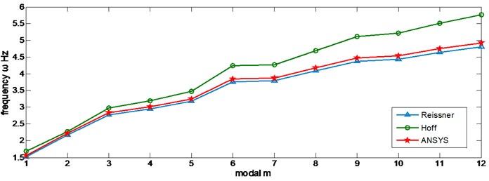
Figure 3 shows that the frequencies obtained by the Resineer theory are much more approximated to the ANSYS result than that obtained by the Hoff theory, and the deviation increases when the order becomes higher. In order to make the analytical results and numerical simulation results consistent, the Resineer theory is chosen as the theoretical basis in the following analysis.

3. The scaling laws of the isotropic sandwich plates

According to the equations of shear strain and rotation [15]:

22

\frac{\partial w}{\partial x} + \frac{\partial u}{\partial z} = β_{x}, \frac{\partial w}{\partial y} + \frac{\partial v}{\partial z} = β_{y},

23

ψ_{x} = \frac{\partial w}{\partial x} - β_{x}, ψ_{y} = \frac{\partial w}{\partial y} - β_{y} .

Substitution of Eq. (22) into Eq. (23) yields:

24

ψ_{x} = - \frac{\partial u}{\partial z}, ψ_{y} = - \frac{\partial v}{\partial z} .

Applying similarity theory to Eq. (22), Eq. (23) and Eq. (24) yields the following scaling laws for $β$ and $ψ$ of the simply supported isotropic sandwich plate:

25

λ_{β_{x}} = \frac{λ_{w}}{λ_{x}} = \frac{λ_{u}}{λ_{z}}, λ_{β_{y}} = \frac{λ_{w}}{λ_{y}} = \frac{λ_{v}}{λ_{z}}, λ_{ψ_{x}} = \frac{λ_{u}}{λ_{z}}, λ_{ψ_{y}} = \frac{λ_{v}}{λ_{z}} .

The equations of the in-plane displacements $u$ , $v$ are obtained by the assumptions (iii) and (iv) of the Reissner theory [15]:

26

\{\begin{matrix} u = \mp \frac{h + t_{h}}{2} ψ_{x} - (z \mp \frac{h + t_{h}}{2}) \frac{\partial w}{\partial x}, \\ v = \mp \frac{h + t_{h}}{2} ψ_{y} - (z \mp \frac{h + t_{h}}{2}) \frac{\partial w}{\partial y} . \end{matrix}

Substitute the Eq. (24) into Eq. (26) yields:

27

\{\begin{matrix} u = \pm \frac{h + t_{h}}{2} \frac{\partial u}{\partial z} - (z \mp \frac{h + t_{h}}{2}) \frac{\partial w}{\partial x}, \\ v = \pm \frac{h + t_{h}}{2} \frac{\partial v}{\partial z} - (z \mp \frac{h + t_{h}}{2}) \frac{\partial w}{\partial y} . \end{matrix}

From Eq. (27), the scale factors must satisfy the following conditions:

28

λ_{u} = λ_{h} \frac{λ_{u}}{λ_{z}} = λ_{z} \frac{λ_{w}}{λ_{x}} = λ_{h} \frac{λ_{w}}{λ_{x}}, λ_{v} = λ_{h} \frac{λ_{v}}{λ_{z}} = λ_{z} \frac{λ_{w}}{λ_{y}} = λ_{h} \frac{λ_{w}}{λ_{y}} .

Those yield the following scaling laws:

29

λ_{h} = λ_{z}, λ_{u} = \frac{λ_{z} λ_{w}}{λ_{x}}, λ_{v} = \frac{λ_{z} λ_{w}}{λ_{y}} .

3.1. Scaling laws of complete geometric similarity

Replace $u$ , $v$ by the functions $U (x)$ , $V (y)$ , then:

30

\{\begin{matrix} u = (A \cos \bar{ω} t + B \sin \bar{ω} t) U (x), \\ v = (A \cos \bar{ω} t + B si n \bar{ω} t) V (y) . \end{matrix}

Substitution of Eq. (30) into Eq. (27) leads to:

31

\{\begin{matrix} U (x) = \pm \frac{h + t_{h}}{2} \frac{\partial U (x)}{\partial z} - (z \mp \frac{h + t_{h}}{2}) \frac{\partial W (x, y)}{\partial x}, \\ V (y) = \pm \frac{h + t_{h}}{2} \frac{\partial V (y)}{\partial z} - (z \mp \frac{h + t_{h}}{2}) \frac{\partial W (x, y)}{\partial y} . \end{matrix}

The following scaling laws can be obtained:

32

λ_{h} = λ_{z}, λ_{U (x)} = \frac{λ_{z} λ_{W (x, y)}}{λ_{x}}, λ_{V (y)} = \frac{λ_{z} λ_{W (x, y)}}{λ_{y}} .

Substitution of Eqs. (22), (23) and (31) into Eq. (3) yields:

33

K_{C} (\frac{\partial^{2} W (x, y)}{\partial x^{2}} + \frac{\partial^{2} W (x, y)}{\partial y^{2}} - \frac{\partial U (x)}{\partial x \partial z} - \frac{\partial V (y)}{\partial y \partial z}) + ρ {\bar{ω}}^{2} W (x, y) = 0 .

From Eq. (33), we obtain:

34

\frac{λ_{K_{C}} λ_{W (x, y)}}{λ_{x}^{2}} = \frac{λ_{K_{C}} λ_{W (x, y)}}{λ_{y}^{2}} = \frac{λ_{K_{C}} λ_{U (x)}}{λ_{x} λ_{z}} = \frac{λ_{K_{C}} λ_{V (y)}}{λ_{y} λ_{z}} = λ_{ρ} {λ_{\bar{ω}}^{2} λ}_{W (x, y)} .

Substitution of Eq. (32) into Eq. (34) yields:

35

\frac{λ_{K_{C}}}{λ_{x}^{2}} = \frac{λ_{K_{C}}}{{λ_{y}}^{2}} = λ_{ρ} λ_{\bar{ω}}^{2} .

Because models have the same material properties as their prototype, the following scaling laws must be satisfied:

36

λ_{K_{C}} = λ_{h} .

It is assumed that $λ_{x} = λ_{y} = λ_{z} = λ_{a} = λ_{b} = λ_{h}$ and $λ_{ρ} = λ_{h},$ the complete geometric similarity conditions in Eq. (35) are simplified as:

37

λ_{\bar{ω}}^{2} = \frac{1}{{λ_{b}}^{2}} .

3.2. Scaling laws of incomplete geometric similarity

When models have the incomplete geometric similarity parameters: $λ_{a} \neq λ_{b},$ $λ_{x} = λ_{a}$ and $λ_{y} = λ_{b}$ and it is supposed that $λ_{a} = C λ_{b}$ , $λ_{h} = A$ , where $C > 0$ and $A$ is a constant, Eq. (35) becomes:

38

\frac{λ_{K_{C}}}{C^{2} λ_{b}^{2}} \neq \frac{λ_{K_{C}}}{λ_{b}^{2}} = λ_{ρ} λ_{\bar{ω}}^{2} .

There are two choices in Eq. (38):

39

\{\begin{array}{l} λ_{ρ} {λ_{\bar{ω}}}^{2} = \frac{A}{C^{2} λ_{b}^{2}}, \\ λ_{ρ} {λ_{\bar{ω}}}^{2} = \frac{A}{λ_{b}^{2}} . \end{array}

Then, the scaling laws of natural frequency are deduced as follows:

40a

λ_{\bar{ω}}^{2} = \frac{1}{C^{2} λ_{b}^{2}},

40b

λ_{\bar{ω}}^{2} = \frac{1}{λ_{b}^{2}} .

Material properties and geometric parameters of the prototype are the same with the example in section 2.3, as shown Table 3. Table 4 shows 7 incomplete geometric similarity models which all have the same material properties with the prototype.

Table 4The parameters of incomplete geometric similarity models

Model	$a$ (m)	$λ_{a}$	$b$ (m)	$λ_{b}$	$C$	$h$ (m)	$t_{h}$ (m)	$λ_{h} = λ_{t_{h}}$
M1	3	5	0.2	50	0.1	0.005	0.0005	20
M2	0.6	25	0.2	50	0.5	0.005	0.0005	20
M3	0.3	50	0.2	50	1	0.005	0.0005	20
M4	0.2	75	0.2	50	1.5	0.005	0.0005	20
M5	0.15	100	0.2	50	2	0.005	0.0005	20
M6	0.075	200	0.2	50	4	0.005	0.0005	20
M7	0.06	250	0.2	50	5	0.005	0.0005	20

3.3. Scaling laws and structure size intervals of first-order natural frequency

According to ANSYS calculation results, the first-order natural frequency is ${\bar{ω}}_{P} = 1.56 Hz$ . Table 5 lists the predicted frequency for models with the two scaling laws in Eq. (40) and the discrepancies between the predicted frequencies and the prototype frequencies.

According to Table 5, the applicable interval possibly exists within the range of M1~M4 under Eq. (40b), but, Eq. (40a) is more sensitive in discrepancy. So in this case, scaling laws Eq. (40b) is satisfied.

Table 5Predicted frequency and discrepancy

Model	Predicted by Eq. (40a) (Hz)	Discrepancy $η$	Predicted by Eq. (40b) (Hz)	Discrepancy $η$
M1	0.136	91.3 %	1.358	13 %
M2	0.715	54.2 %	1.43	8.3 %
M3	1.63	4.8 %	1.63	4.8 %
M4	2.893	85.5 %	1.929	23.6 %
M5	4.554	192 %	2.277	46 %
M6	15.615	901 %	3.904	150.2 %
M7	23.87	1429.8 %	4.77	206 %

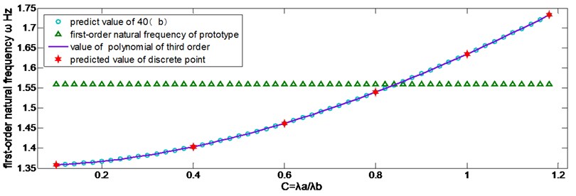
When $C = 1.2$ , the predicted frequency is ${\bar{ω}}_{P r} = 1.755$ and the corresponding discrepancy is $η = 12.5 %.$ So the first-order natural frequency is predicted as six discrete values $C = [0.1, 0.4, 0.6, 0.8, 1.0, 1.2]$ are taken within the range of $\in [0.1, 1.2]$ . Then the relationship between the first-order natural frequency and $C$ can be determined by fitting a third order polynomial, the result is as follows:

41

{\bar{ω}}_{P r} = - 0.055 C^{3} + 0.343 C^{2} - 0.008 C + 1.355 .

The first-order natural frequency is obtained by different methods and plotted in Figure 4. Here the range of $C$ is $[0.1, 1.2]$ , its step size is 0.02. It can be seen from Figure 4 that the values obtained from third order polynomial fit the curve well.

Fig. 4Curve of predicted value and its verification

By introducing a $±10 %$ discrepancy of $η$ , the acceptable range of $C$ are calculated as:

42

η = \frac{|（- 0.055 C^{3} + 0.343 C^{2} - 0.008 C + 1.355 - 1.56）|}{1.56} = 0.1 .

The roots of Eq. (42) in the interval $C \in [0.1, 1.2]$ are $C_{m i n} = 0.40$ and $C_{m a x} = 1.15$ .

So Eq. (40b) is chosen as scaling laws within the interval $C \in [0.40, 1.15]$ . If $λ_{b}$ and $λ_{h}$ are close enough, the intervals $C$ will be wider.

3.4. Scaling laws and structure size intervals of high-order natural frequencies

According to the scaling law Eq. (40b), there are the same mode shapes between similar model and prototype, the predicted values of high-order natural frequencies and the discrepancies are shown in Table 6.

Table 6Predicted values and the discrepancies of the revised applicable intervals

Order	Mode shape $(m, n)$	$C = 0.40$ Mode shape $(m, n)$	$C = 1.15$ Mode shape $(m, n)$	Revised applicable intervals	Predicted values	Discrepancy $η$
1	(1, 1)	(1, 1)	(1, 1)	–	–	–
2	(2, 1)	(2, 1)	(2, 1)	[0.82, 1.1]	(2.02, 2.43)	(9.1 %, 9.3 %)
3	(1, 2)	(3, 1)	(1, 2)	[0.92, 1.1]	(2.86, 2.92)	(0.8 %, 2.6 %)
4	(3, 1)	(4, 1)	(3, 1)	[0.92, 1.1]	(2.87, 3.31)	(5.1 %, 9.6 %)
5	(2, 2)	(5, 1)	(2, 2)	[0.92, 1.1]	(3.21, 3.4)	(1.1 %, 4.6 %)
6	(3, 2)	(6, 1)	(3, 2)	[1, 1.1]	(3.88, 4.08)	(0.97 %, 6.2 %)
7	(4, 1)	(1, 2)	(4, 1)	[1, 1.1]	(3.9, 4.23)	(0.89 %, 9.4 %)

Table 6 demonstrates that when the order gets higher and the mode shape changes, the applicable structure size intervals become narrow and closer to the complete geometric similarity conditions, but it is still incomplete geometric similarity model because of $λ_{h} \neq λ_{b}$ .

4. The scaling laws and structure size intervals of harmonic response

When the isotropic sandwich plate in Figure 1 is subjected to the harmonic excitation $q (t) = q \sin ({\bar{ω}}_{q} t)$ on the geometric center, where $q$ is the amplitude of pressure, the force applied to the plate is $F (t) = q d x d y \sin ({\bar{ω}}_{q} t)$ , where $d x$ , $d y$ are the length and width of the excited element respectively.

In this section, the scaling laws and applicable intervals of the response will be determined when the isotropic sandwich plate is suffering the harmonic excitation. After this, the amplitude-versus-frequency curve of prototype is predicted by the model experiments.

4.1. Scaling laws of complete geometric similarity

The dimensional analysis method [16] is applied to calculate the $π$ term and determine two scaling laws:

43

λ_{\bar{ω}} = \frac{1}{λ_{t}}, λ_{{\bar{ω}}_{q}} = \frac{1}{λ_{t}} .

Substitution of Eq. (43) into Eq. (3) yields:

44

\frac{λ_{K_{C}} λ_{w}}{λ_{x}^{2}} = \frac{λ_{K_{C}} λ_{w}}{λ_{y}^{2}} = \frac{λ_{K_{C}} λ_{u}}{λ_{x} λ_{z}} = \frac{λ_{K_{C}} λ_{v}}{λ_{y} λ_{z}} = λ_{ρ} {λ_{\bar{ω}}^{2} λ}_{w} = λ_{q} .

According to Eq. (36), Eq. (44) and the condition of complete geometric similarity $λ_{u} = λ_{v} = λ_{x} = λ_{y} = λ_{z} = λ_{a} = λ_{b} = λ_{h} = λ_{ρ},$ and $λ_{\bar{ω}} = λ_{{\bar{ω}}_{q}},$ the scaling laws of complete geometric similarity are:

45

λ_{q} = λ_{b} {λ_{\bar{ω}}^{2} λ}_{w} = \frac{λ_{w}}{λ_{b}} .

When the frequency’s scaling law of complete geometric similarity $λ_{\bar{ω}}^{2} = 1 / λ_{b}^{2}$ is considered, Eq. (45) can be simplified as:

46

λ_{w} = \frac{λ_{q}}{λ_{b} λ_{\bar{ω}}^{2}} = λ_{q} λ_{b} .

And the complete scaling laws of harmonic excitation response are:

47

\{\begin{array}{l} λ_{\bar{ω}}^{2} = \frac{1}{λ_{b}^{2}}, \\ λ_{w} = λ_{q} λ_{b} . \end{array}

Eq. (47) gives the same results with Ref. [6]. It is worthy of note that according to Ref. [6], Eq. (47) can be applied not only to the harmonic response, but also to other responses of random excitation $q (x, y, t)$ .

4.2. Scaling laws of incomplete geometric similarity

If the model cannot satisfy the complete conditions, there are $λ_{x} = λ_{a}$ , $λ_{y} = λ_{b}$ , $λ_{a} \neq λ_{b}$ , it is supposed $λ_{a} = C λ_{b}$ and $λ_{h} = A$ where $A$ is constant, substitution of these laws into Eq. (44) yields:

48

\frac{λ_{K_{C}} λ_{w}}{{C^{2} λ}_{b}^{2}} \neq \frac{λ_{K_{C}} λ_{w}}{{λ_{b}}^{2}} \neq \frac{λ_{K_{C}} λ_{u}}{{C λ}_{b} λ_{z}} \neq \frac{λ_{K_{C}} λ_{v}}{λ_{b} λ_{z}} = λ_{ρ} {λ_{\bar{ω}}^{2} λ}_{w} = λ_{q} .

Substitution of Eqs. (28) and (36) into Eq. (48) yields:

49

\frac{A λ_{w}}{{C^{2} λ}_{b}^{2}} \neq \frac{A λ_{w}}{λ_{b}^{2}} \neq \frac{A^{3} λ_{w}}{C^{4} λ_{b}^{4}} \neq \frac{A^{3} λ_{w}}{{C^{2} λ}_{b}^{4}} \neq \frac{A^{3} λ_{w}}{λ_{b}^{4}} = A {λ_{\bar{ω}}^{2} λ}_{w} = λ_{q} .

So the scaling laws of the amplitude are as follows:

50

λ_{w} = \frac{λ_{q}}{A λ_{\bar{ω}}^{2}} = \frac{λ_{b}^{2} λ_{q}}{A} .

In allusion to Eq. (50), the following matters should be consideres.

(1) Eq. (50) should satisfy the interval requirement $C \in [0.40, 1.15]$ .

(2) Though the harmonic excitation is a concentrated load, it has the infinitesimal area $S = d x d y$ which is subjected to the pressure $q$ , so there are the scaling laws of area $S$ : $λ_{S} = {C λ}_{b}^{2}$ , and the force $λ_{F} = {C λ}_{b}^{2} λ_{q}$ . Eq. (49) can be simplified as:

51

λ_{w} = \frac{λ_{F}}{C A},

where the subscript $F$ represents the force amplitude.

(3) $λ_{{\bar{ω}}_{q}} = λ_{\bar{ω}}$ should be hold, which is the same as that in complete geometric similarity.

4.3. Verify the scaling laws and the applicable intervals

In order to verify the scaling laws and the applicable intervals, the same isotropic sandwich plate as that in section 2.3 is considered. When the excitation is with $λ_{F} = 10$ , the excitation of prototype is $F = 100 \sin ({\bar{ω}}_{q} t)$ , the first-order amplitude-versus-frequency curve in the interval $C \in [0.40, 1.1 5]$ is predicted in this section.

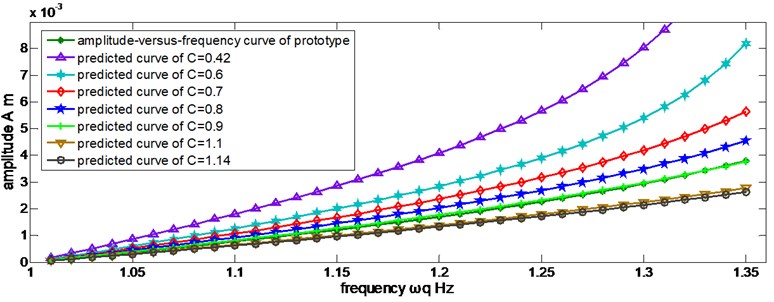
The distorted scaling laws may cause the extreme difference between the discrepancy and natural frequency of prototype and those of the predicted value, so the amplitude discrepancy near the resonance point will be amplified. When the frequency is away from the resonance zone, the predicted amplitudes in different $C$ are displayed in Figure 5.

Figure 5 indicates that Eq. (51) is not applicable in $C \in [0.40, 1.15]$ , so a revised scaling law is needed. Eq. (51) is multiplied by a correction factor $C$ , where $C = λ_{a} / λ_{b}$ , then:

52

λ_{w} = \frac{λ_{F}}{A} .

Fig. 5Predicted amplitudes in different discrete values of C by Eq. (51)

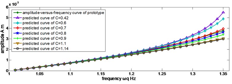
The new predicted curves are shown in Figure 6.

Figure 6 shows that Eq. (52) is an applicable scaling law of the amplitude. The discrepancies increase as the frequency rises because of the discrepancy of natural frequency, which was mentioned in previous section, and the applicable structure size intervals is uniform, $C \in [0.40, 1.15]$ .

Fig. 6Predicted amplitudes in different discrete values of C by Eq. (52)

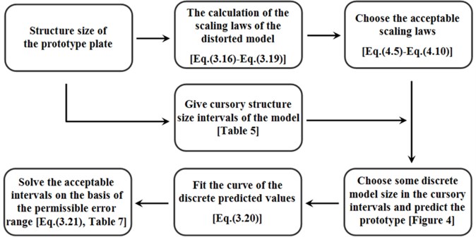
5. Flow steps of the intervals determination method

The applicable structure size intervals have been investigated above. The flow of the intervals determination method is summarized in Figure 7.

Fig. 7Flow steps of the intervals determination method

6. Conclusion

The Resineer theory of plates was chosen as the basic theory of this paper by comparing with the Hoff theory of plates. The scaling laws of both complete and incomplete geometric similarity model of the isotropic sandwich plates were obtained. The determination method of the structure size interval of the models was studied in the end. Some specific conclusions are listed as follows:

(1) The governing equation and the analytic solution of Hoff theory have the extra terms $D_{f}$ and $k_{f}$ , which indicate the influence of the face sheets’ flexural stiffness of the sandwich plate.

(2) It is verified that analytic result from Reissner theory is more approximated the result from ANSYS, so the modeling of ANSYS sandwich plate element uses the Reissner theory.

(3) Establishing the scaling laws of frequency and dynamic response $λ_{\bar{ω}}^{2} = 1 / λ_{b}^{2},$ $λ_{w} = λ_{F} / C A$ . A correction factor $C$ is used to revise the scaling laws of amplitude: $λ_{w} = λ_{F} / A$ .

(4) Obtaining the predicted curves by using the polynomial of third order, and finding the applicable structure size intervals of each order natural frequency which satisfy the discrepancy $η < 10 %$ .

References

M. John Scaling of impact-loaded carbon-fiber composites. AIAA Journal, Vol. 26, Issue 8, 1988, p. 989-994.

Search CrossRef
J. Rezaeepazhand, G. J. Simitses, J. H.Starnes Scale models for laminated cylindrical shells subjected to axial compression. Composite Structure, Vol. 34, Issue 4, 1996, p. 371-379.

Search CrossRef
J. Rezaeepazhand, G. J. Simitses, J. H.Starnes Design of scaled down models for predicting shell vibration response. Journal of Sound and Vibration, Vol. 195, Issue 2, 1996, p. 301-311.

Search CrossRef
J. Rezaeepazhand, G. J. Simitses Structural similitude for vibration response of laminated cylindrical shells with double curvature. Composites Part B-Engineering, Vol. 28, Issue 3, 1997, p. 195-200.

Search CrossRef
Y. Qian, S. R. Swanson Experimental measurement of impact response in carbon/epoxy plates. AIAA Journal, Vol. 28, Issue 6, 1990, p. 1069-1074.

Search CrossRef
Y. Qian, S. R. Swanson, R. J. Nuismer, et al. An experimental study of scaling rules for impact damage in fiber composites. Journal of Composite Materials, Vol. 24, Issue 5, 1990, p. 559-570.

Search CrossRef
V. Ungbhakorn, P. Singhatanadgid Similitude invariants and scaling laws for buckling experiments on anti-symmetrically isotropic laminated plates subjected to biaxial loading. Composite Structure, Vol. 59, Issue 4, 2003, p. 455-465.

Search CrossRef
P. Singhatanadgid, V. Ungbhakorn Scaling laws for vibration response of anti-symmetrically isotropic laminated plates. Structural Engineering and Mechanics, Vol. 14, Issue 3, 2002, p. 345-364.

Search CrossRef
S. D. Rosa, F. Franco A scaling procedure for the response of an isolated system with high modal overlap factor. Mechanical Systems and Signal Processing, Vol. 22, Issue 7, 2008, p. 1549-1565.

Search CrossRef
E. E. Bachynski, M. R. Motley, Y. L. Young Dynamic hydroelastic scaling of the underwater shock response of composite marine structures. Journal of Applied Mechanics-Transactions of the ASME, Vol. 79, Issue 1, 2012, p. 501-507.

Search CrossRef
J. Rezaeepazhand, A. A. Yazdi Similitude requirements and scaling laws for flutter prediction of angle-ply composite plates. Composites Part B-Engineering, Vol. 42, Issue 1, 2011, p. 51-56.

Search CrossRef
J. Rezaeepazhand, G. J. Simitses, J. H.Starnes Use of scaled-down models for predicting vibration response of isotropic laminated plates. Composite Structure, Vol. 30, Issue 4, 1995, p. 419-426.

Search CrossRef
G. J. Simitses, J. Rezaeepazhand Structural similitude and scaling laws for laminated beam-plates. Springfield Publishers, Washington, 1992.

Search CrossRef
H. C. Hu On some problems of the antisymetrical small deflection of isotropic sandwich plates. Chinese Journal of Theoretical and Applied Mechani, Vol. 6, Issue 1, 1963, p. 53-60.

Search CrossRef
L. A. Carlsson, G. A. Kardomates Structural and failure mechanics of laminated composites. Springer Publishers, Berlin, 2011.

Search CrossRef
H. G. Harris, G. M. Sabnis Structural modeling and experimental techniques. CRC Press, New York, 1999.

Search CrossRef

About this article

Received

08 September 2013

Accepted

16 October 2013

Published

31 March 2014

Keywords

isotropic sandwich plate

scale model

dynamic similarity

size interval

Acknowledgements

This work is supported by National Science Foundation of China (51105064), National Program on Key Basic Research Project (2012CB026000), and Natural Science Foundation of Liaoning Province (201202056).

This is an open access article distributed under the Creative Commons Attribution License, which permits unrestricted use, distribution, and reproduction in any medium, provided the original work is properly cited.