A comparison of different methods for determination of coupling factor and velocity response of coupled plates

Pankaj, Achuthan C.; Sastry, Sridhar; Murigendrappa, S. M.

Journal of Vibroengineering

Browse Journal

Submit article

Published: 31 December 2013

Check for updates

A comparison of different methods for determination of coupling factor and velocity response of coupled plates

Achuthan C. Pankaj¹

Sridhar Sastry²

S. M. Murigendrappa³

¹CSIR-National Aerospace Laboratories, Bangalore, India

^{2, 3, 1}National Institute of Technology Karnataka, Surathkal, India

Corresponding Author:

Achuthan C. Pankaj

Cite the article Download PDF

Downloads 1216

WoS Core Citations 7

Abstract

Coupling loss factors (CLF) and velocity responses has been computed for two plates joined in a ‘L’ junction configuration using Statistical Energy Analysis. The analyses have been carried out to study the effects of internal loss/damping factor on the coupling factors. The effects of plate widths on the coupling factors and velocity responses at high frequencies has also been studied. The statistical energy parameters have been computed using analytical wave approach, finite element method and Free-SEA software. The studies have revealed that the coupling factor computed by the wave approach is independent of the internal loss factor as compared to the values computed using finite element method, wherein CLF increases linearly as the internal loss factor varies from a zero value, followed by a transition region and converges to the values obtained by the analytical wave approach and remains insensitive to changes at higher values of damping. The results obtained from the studies signify the effects of internal loss/damping factor and plate widths on proper selection and usage of the above mentioned methods for the estimation of coupling factors and velocity responses using statistical energy approach.

1. Introduction

Statistical Energy Analysis (SEA) is one of the widely used energy methods, developed in the early 1960s to predict the vibration response of structures at high frequencies [1, 2]. The initial applications were related to aerospace, to predict rocket noise of satellite launch vehicles, wherein the technological improvements leading to lightweight aerospace structures, and high frequency broad-band loads attracted more attention to higher order modal analyses for predicting structural fatigue, equipment failure and noise production. SEA parameters can be computed by analytical wave approach, power injection method [3], experimental approach [4], finite element method or the receptance method [5]. The results for steady state excitation using the power injection method [3] has been found to be in good agreement with the predicted SEA parameters as compared to transient excitation. The method predicting the SEA parameters by power balance equations, wherein proper care has to be taken to avoid ill-conditioning of the matrices due to inversion, is achieved by keeping the values of internal loss factor higher than the coupling loss factor (CLF) to avoid equi-partition of modal energy and satisfy the assumption of weak coupling between the subsystems.

SEA involves predicting the vibration response of a complex structure by dividing it into a number of subsystems, and is characterized by mean energy per mode. The change in energy level between subsystems is characterized by internal and coupling loss factors. Internal loss factor corresponds to damping factor in the subsystem itself and CLF corresponds to the energy dissipation during flow across the subsystems. Coupling loss and internal loss/damping factors constitute a matrix of energy balance equations, which is used to compute the energies by the power balance approach, once the power inputs are known. The CLFs can be obtained using analytical wave approaches from coefficients of energy propagation, via junctions of subsystems, known for several types of junctions like L, T, and X-junction [6] for semi-infinite beams/plates. Alternatively, the values can also be found by the power injection approach after computing the energies and power inputs through experiments or finite element analysis.

In this paper comparisons have been made for the computed coupling factors and velocity responses for an ‘L’ shaped junction between two sub-systems, by modeling it as two beams/plates at right angles using analytical wave approach, finite element method and Free-SEA software [7]. The effects of internal loss/damping factor on the computed coupling factors have been studied. It has been observed that though the coupling factor is independent of internal loss/damping factor according to classical SEA wave approach [8], it varies linearly with change in internal loss factor/damping factor at lower damping values, as computed using modal approach by the finite element method. The effect of plate widths on the computed coupling factors and velocity responses for the configuration has also been studied.

2. Statistical energy analysis

SEA derives its principles based on the first law of thermodynamics of conservation of energy. The system under consideration is divided into subsystems with the usual aim to predict the vibrational energy level of each subsystem, which is obtained by establishing a set of power balance equations, based on the assumption that the energy flow between two connected subsystems is proportional to the difference in the subsystem modal energies. Assuming power input injected to an independent single subsystem, i.e. not connected to other subsystems, the subsystem would vibrate with energy $E$ with a power loss only due to dissipation, associated with vibrational energy by the damping loss factor $η$ , that can be expressed as:

1

{\bar{P}}_{i, i n} = {\bar{P}}_{i, d i s s} = ω η 〈\bar{E}〉,

where, ${\bar{P}}_{i, i n}$ – Power injected in subsystem $i$ , $〈 \bar{E} 〉$ – Frequency averaged energy in subsystem $i$ , $η$ – Structural damping loss factor, $〈 〉$ – indicates spatial averaging, and bar indicates frequency averaging.

In case of two coupled subsystems (Fig. 1), there is a power exchange among the coupled subsystems, resulting in energy loss in the form of vibrational energy from one subsystem and corresponding gain of the energy by the other connected subsystem.

Fig. 1Energy flow across two subsystems

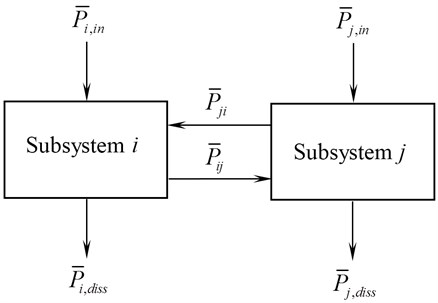
The power balance equation is given by:

2

{\bar{P}}_{i, i n} = {\bar{P}}_{i, d i s s} + {\bar{P}}_{i j},

3

{\bar{P}}_{j, i n} = {\bar{P}}_{j, d i s s} + {\bar{P}}_{j i},

where the power transmitted between subsystem $i$ and $j$ is given by:

4

{\bar{P}}_{i j} = ω η_{i j} 〈 {\bar{E}}_{i} 〉 - ω η_{j i} 〈 {\bar{E}}_{j} 〉,

5

{\bar{P}}_{j i} = ω η_{j i} 〈{\bar{E}}_{j}〉 - ω η_{i j} 〈{\bar{E}}_{i}〉 .

The CLFs ( $η_{i j}$ and $η_{j i}$ ) have been included in the Eqs. (4) and (5). The power balance equation can be further simplified as:

6

{\bar{P}}_{i, i n} = ω η_{i} 〈{\bar{E}}_{i}〉 + ω η_{i j} 〈{\bar{E}}_{i}〉 - ω η_{j i} 〈{\bar{E}}_{j}〉,

7

{\bar{P}}_{j, i n} = ω η_{j} 〈{\bar{E}}_{j}〉 + ω η_{j i} 〈{\bar{E}}_{j}〉 - ω η_{i j} 〈{\bar{E}}_{i}〉,

where, $ω$ – central band frequency, $η_{i}$ – internal damping loss factor in subsystem $i$ , $η_{i j}$ – CLF from subsystem $i$ to subsystem $j$ , $η_{j i}$ – CLF from subsystem $j$ to subsystem $i$ , $〈{\bar{E}}_{i}〉$ – frequency averaged energy in subsystem $i$ , $〈{\bar{E}}_{j}〉$ – frequency averaged energy in subsystem $j$ .

The power balance equation can be further related by defining new set of coefficients, called the power transfer coefficients (modal coupling factors) [2, 9]:

8

M_{i j} = η_{i j} ω n_{i} = η_{j i} ω n_{j} = M_{j i},

where $n_{i}$ and $n_{j}$ are the modal density of subsystem $i$ and $j$ respectively.

Assuming modal energy in both subsystems $i$ and $j$ are same, i.e. equipartition of modal energies in both subsystems $i$ and $j$ [4, 8], then:

9

n_{i} η_{i j} = n_{j} η_{j i},

the power balance equation reduces to:

10

{\bar{P}}_{i, i n} = ω η_{i} 〈{\bar{E}}_{i}〉 + ω η_{i j} n_{i} (\frac{〈{\bar{E}}_{i}〉}{n_{i}} - \frac{〈{\bar{E}}_{j}〉}{n_{j}}),

11

{\bar{P}}_{j, i n} = ω η_{j} 〈{\bar{E}}_{j}〉 + ω η_{j i} n_{j} (\frac{〈{\bar{E}}_{j}〉}{n_{j}} - \frac{〈{\bar{E}}_{i}〉}{n_{i}}),

where $\frac{〈 {\bar{E}}_{i} 〉}{n_{i}}$ and $\frac{〈 {\bar{E}}_{j} 〉}{n_{j}}$ are the modal energy (energy per mode) of subsystem $i$ and $j$ respectively.

Similarly for $n$ subsystems the power balance equation can be given by:

12

ω [\begin{matrix} (η_{1} + \sum_{i \neq 1}^{N} η_{1 i}) n_{1} & - η_{12} n_{1} & \dots & - η_{1 N} n_{1} \\ - η_{21} n_{2} & (η_{2} + \sum_{i \neq 2}^{N} η_{2 i}) n_{2} & \dots & - η_{2 N} n_{2} \\ ⋮ & ⋮ & ⋱ & ⋮ \\ - η_{N 1} n_{N} & \dots & \dots & (η_{N} + \sum_{i \neq N}^{N - 1} η_{N i}) n_{N} \end{matrix}] \times [\begin{matrix} \frac{〈{\bar{E}}_{1}〉}{n_{1}} \\ \frac{〈{\bar{E}}_{2}〉}{n_{2}} \\ ⋮ \\ \frac{〈{\bar{E}}_{N}〉}{n_{N}} \end{matrix}] = [\begin{matrix} {\bar{P}}_{i, 1} \\ {\bar{P}}_{i, 2} \\ ⋮ \\ {\bar{P}}_{i, N} \end{matrix}] .

In predictive SEA, coupling and damping loss factors are estimated through experiments, analytical or numerical approaches by solving the power balance equations for the unknown’s i.e. the energies of subsystems [6, 10]. In case of experimental SEA, power is injected to each subsystem in the structure in turn by means of a hammer, a shaker or a loudspeaker. Then, each time the energy in each subsystem is measured (by accelerometers or microphones). Once the energies in all the subsystems are computed for the corresponding power to the respective sub-systems, with known material damping, the coupling factors in Eq. (12) can be found out by the matrix inversion approach.

3. Analysis and procedure

The coupling factor and velocity responses for two thin plates joined by ‘L’ junction (Fig. 2) has been analyzed by using analytical wave approach, finite element method and Free-SEA software. The material properties assumed for the configurations are given in Table 1. The length of each beam/plate has been assumed to be 1.0 m with a thickness of 2 mm. Pinned boundary conditions have been assumed both the beams/plates near the ‘L’ junction. The analyses have been carried out to study the effect of internal loss/damping factor on the CLF for the configuration by varying the internal loss factor in the range of 0.00001 to 0.04, for a width of 0.01 m for beam and 0.9 m for the plate configuration. In addition studies have also been carried out to estimate the coupling factors and velocity responses for different widths, varying from 0.0025 m to 0.1 m for the beam and 0.01 m to 0.9 m for the plate with a constant value of internal loss factor of 0.04.

Fig. 2Two plates coupled at right angles

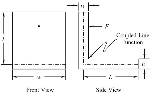
Table 1Material and geometrical specifications

Internal damping	$η_{1} = η_{2} =$	0.00001 to 0.04
Width	$w =$	$\{\begin{array}{l} 0.0025 m t o 0.1 m (B e a m) \\ 0.01 m t o 0.9 m (P l a t e) \end{array}$
Length	$L =$	1.0 m
Thickness	$t_{1} = t_{2} =$	2 mm
Density	$ρ =$	7800 kg/m³
Poisson’s ratio	$υ =$	0.3
Young’s modulus	$E =$	200 GPa
Force	$F =$	1 N
Frequency	$f =$	1000 to 8000 Hz

A brief description of the applied methods has been explained in the following sections.

3.1. Analytical wave approach for plates

The subsystems in consideration have been analyzed for flexural waves, which plays an important role for vibrations at high frequencies and sound radiation. The CLF $η_{12}$ between two plates for a line junction is given by [11, 12]:

13

η_{12} = \frac{2 C_{B} L τ_{12}}{π ω A},

where $ω$ is the angular forcing frequency, $A$ is the surface area, $w$ is the length of the junction of the two plates and $C_{B}$ is the bending wave speed of the first plate for two connected plates as the function of center frequency, $f$ given by:

14

C_{B} = \sqrt{1.8 C_{L} t f} .

$τ_{12}$ is the wave transmission coefficient defined as the ratio of transmitted power to the incident power. The wave transmission coefficient for random incidence vibrational energy of two coupled plates at right angles to each other can be calculated by the approximate formula as:

15

τ_{12} = τ_{12} (0) \frac{2.754 X}{1 + 3.24 X},

where, $X$ is the ratio of plate thicknesses.

The normal transmission coefficient $τ_{12} (0)$ may be calculated as:

16

τ_{12} (0) = 2 {(ψ^{\frac{1}{2}} + ψ^{- \frac{1}{2}})}^{- 2},

where, $ψ = \frac{ρ_{1} C_{L 1}^{\frac{3}{2}} t_{1}^{\frac{5}{2}}}{ρ_{2} C_{L 2}^{\frac{3}{2}} t_{2}^{\frac{5}{2}}}$ .

The modal density of flat plate in flexural vibration is given by:

17

n (ω) = \frac{A \sqrt{12}}{2 π C_{L} t},

where longitudinal wave speed is given by:

18

C_{L} = \sqrt{\frac{E}{ρ (1 - υ^{2})}} .

$E$ is the Young’s modulus, $υ$ is the Poisson’s ratio, $A$ is the surface area and $t$ the thickness of the plate under consideration. The time averaged power input for a unit force $F$ is given by:

19

P_{i n} = \frac{1}{2} {|\tilde{F}|}^{2} R e \{{\tilde{Z}}_{m}^{- 1}\} .

The real part of drive-point mechanical impedance of an infinite plate of thickness $t$ and mass per unit area $ρ_{a}$ in flexural vibration is given by:

20

R e \{{\tilde{Z}}_{m}^{- 1}\} = 8 \sqrt{\frac{E t^{3} ρ_{a}}{12 (1 - υ^{2})}} .

The forcing frequencies are in the range of 0-8000 Hz. The energies in each subsystem can be computed by the matrix inversion approach from Eq. (12) after computation of power input and coupling factor. The maximum velocity response $V_{i}$ of each subsystem can be obtained from the obtained energy $E_{i}$ under a particular power input by Eq. (20):

21

V_{i} = \sqrt{\frac{2 E_{i}}{M}} .

3.2. Analytical wave approach for beams

The CLF for two beams joined at right angles to each other in terms of transmission coefficient $τ_{12}$ is given by [13]:

22

η_{i j} = \frac{C_{B i} τ_{i j}}{ω L_{i}},

where the bending wave speed is given by:

23

C_{B i} = \sqrt{\frac{ω^{4} E_{i} I_{i}}{ρ_{i} A_{i}}},

where $L_{i}$ is the length of the beam $i$ under consideration, $ω$ is the angular forcing frequency and $C_{B i}$ is the sound speed of flexural waves, $E_{i}$ is the Young’s modulus, $I_{i}$ is the second moment of area, $ρ_{i}$ is the density and $A_{i}$ is the cross-sectional area. The transmission coefficient across the joint relating the incident waves in subsystem $i$ to be transmitted in subsystem $j$ for the flexural wave may be computed as:

24

τ_{i j} = \frac{2 β^{2} + 1}{9 β^{2} + 6 β + 2},

where:

25

β = \frac{C_{L i}}{C_{B i}},

and the longitudinal wave speed for beam is given by:

26

C_{L} = \sqrt{\frac{E}{ρ}} .

The time averaged power input for a unit force $F$ is obtained as:

27

P_{i n} = \frac{1}{2} {|\tilde{F}|}^{2} R e \{{\tilde{Z}}_{m}^{- 1}\} .

The real part of drive-point mechanical impedance of an infinite beam of thickness ( $t$ ), cross-sectional area ( $A$ ) and density ( $ρ$ ) in flexural vibration for an end loading is given by [11]:

28

R e \{{\tilde{Z}}_{m}^{- 1}\} = 2.67 ρ A \sqrt{C_{L} t f},

and:

29

R e {{\tilde{Z}}_{m}^{- 1}} = 0.67 ρ A \sqrt{C_{L} t f},

for central loading respectively. The forcing frequencies are in the range of 0-8000 Hz. The energies in each subsystem can be computed by the matrix inversion approach from Eq. (12) after computation of power inputs and coupling factor. The maximum velocity response $V_{i}$ of each subsystem can be computed from the energy $E_{i}$ under a particular power input, i.e.:

30

V_{i} = \sqrt{\frac{2 E_{i}}{M}} .

The coupling factors and velocity responses have been computed by in-house program built using the analytical wave approach as discussed above, in MATLAB software.

3.3. Finite element analysis

The finite element analysis using the modal approach has been carried out using Ansys Software [14]. In numerical methods the behavior of SEA parameters with change in inputs (geometry, boundary conditions and damping) for the given structure can be modeled easily and is less time consuming as compared with the experimentation of the real structure. The other advantages of numerical method include cost efficiency and flexibility. In case of beam elements, the configuration under consideration has been modeled using 200 beam3 elements (Fig. 3). Beam 3 is a uni-axial element with tension, compression, and bending capabilities. The element has three degrees of freedom at each node: translations in the nodal $x$ and $y$ directions and rotation about the nodal $z$ -axis.

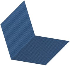
The same structure has also been modeled using shell 63 elements with a size of 0.01 m for the configuration with plate width of 0.9 m and a size of 0.02 m for the rest of the considered configurations (Fig. 4) with pinned boundary conditions. Shell63 has both bending and membrane capabilities. Both in-plane and normal loads are permitted. The element has six degrees of freedom at each node: translations in the nodal $x$ , $y$ and $z$ directions and rotations about the nodal $x$ , $y$ , and $z$ -axes.

A harmonic force with unit load intensity has been applied in the range of frequencies of 0-8000 Hz. The load has been applied on one beam/plate and the velocity responses on both the beams/plates were computed. Macros have been developed in Ansys Parametric Design language (APDL) for automating the computation of energy ( $E_{i}$ ) of each subsystem with mass ( $M_{i}$ ) and maximum subsystem velocity ( $V_{i}$ ) according to Eq. (12). Spatial energy average has been obtained by loading each subsystem at 25 %, 50 %, 75 % and 100 % of its length:

31

E_{i} = \frac{M_{i} V_{i}^{2}}{2} .

Fig. 3Finite element model (beam elements)

Fig. 4Finite element model (shell elements)

The coupling factors are computed by the matrix inversion approach from Eq. (12) after computation of power inputs and corresponding energies in all the subsystems. The maximum average velocity response $V_{i}$ of each subsystem can be obtained directly from the post-processing of the output results.

3.4. Free-SEA software

Free SEA is a free software running under Win32, developed as a result of several SEA codes used in research work, by Dr. Ennes Sarradj at Technische Universität, Dresden [7]. It implements the SEA – for the calculation of high frequency air- and structure-borne sound. The software is available free of charge and may be used for educational purposes, non-commercial and commercial research as long the user accepts the terms and conditions of the license as stated by the author. The coupling factors and velocity responses for the two plates joined at right angles obtained from the above – mentioned methods for different cases has been compared with the results obtained through Free SEA software in the results section.

4. Results and discussion

The variation of CLF against frequencies, for a width of 0.01 m and internal loss factor of 0.04 has been shown in Table 2 and Fig. 5 for the beam formulation. The same has been shown using the plate formulation for a plate width of 0.9 m and internal loss factor of 0.04 in Table 3 and Fig. 6. The frequency averaged coupling factors computed by both of the methods are in good agreement.

Table 2Variation of coupling factor v/s frequencies for the beam

Frequency (Hz)	Coupling Loss Factor
Frequency (Hz)	Analytical	FEM
1000	0.0050	0.000171
2000	0.0034	0.003185
3000	0.0027	0.003420
4000	0.0023	0.001785
5000	0.0020	0.001800
6000	0.0018	0.003060
7000	0.0017	0.001062
8000	0.0015	0.001831
Average	0.0025	0.002310

Table 3Variation of coupling factor vs frequencies for the plate

Frequency (Hz)	Coupling Loss Factor
Frequency (Hz)	Analytical	FEM	Free-SEA Software
1000	0.0046	0.006268	0.004709
2000	0.0032	0.005084	0.00326
3000	0.0026	0.001899	0.002682
4000	0.0023	0.001878	0.002277
5000	0.0020	0.001196	0.002036
6000	0.0019	0.000986	0.001848
7000	0.0017	0.000804	0.001687
8000	0.0016	0.000746	0.001545
Average	0.0025	0.002359	0.002505

The CLF obtained using the analytical wave approach for beam and plate is insensitive to the variation in internal loss factor. The CLF computed using finite element method increases linearly as the internal loss factor varies from a zero value, followed by a transition region and converges to the values obtained by the analytical wave approach and remains insensitive to changes at higher values of damping (Fig. 7, 8) for both beam and plate formulation. The observed results are in agreement with similar studies carried out by Woodhouse [8] for simply supported coupled beams and plates.

Fig. 5Variation of coupling loss factor vs frequencies for beam

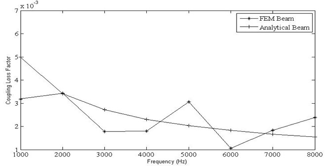
Fig. 6Variation of coupling loss factor vs frequencies for plate

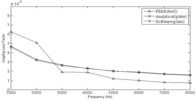
Fig. 7Variation of coupling factor with internal loss factor for beam

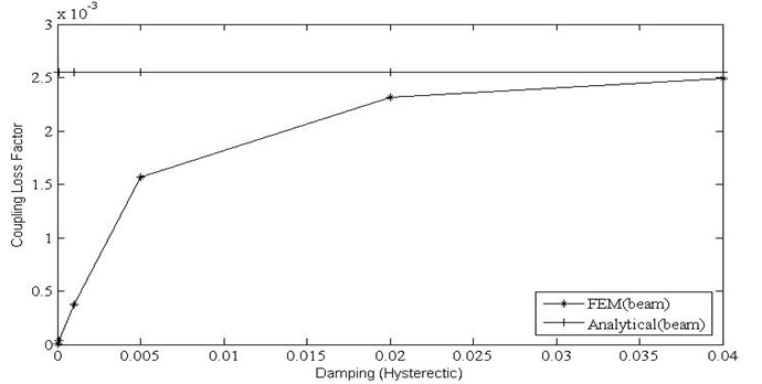
Fig. 8Variation of coupling factor with internal loss factor for plate

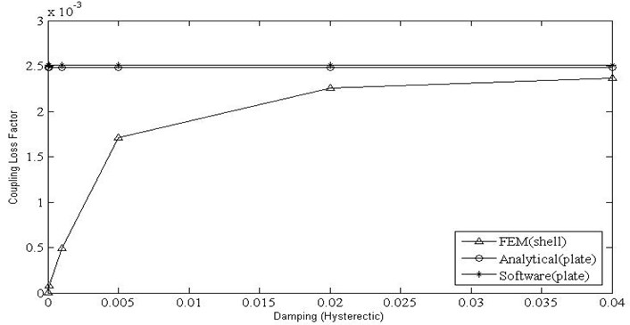
Fig. 9Variation of coupling factor with width for beam

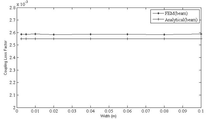
Fig. 10Variation of coupling factor with width for shell

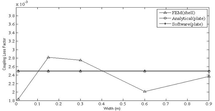
The variation of CLF with variation in width for the beam and plate has been plotted in Fig. 9 and Fig. 10. The values computed by analytical wave approach for both beam and plates are independent of the change in width. The CLF computed for beam using the finite element method is in agreement with the analytical values. It is evident (Fig. 10) that, the variation of the CLF obtained by finite element method, analytical method and Free-SEA software is high, but as the width increases it converges, where the plate theory is valid.

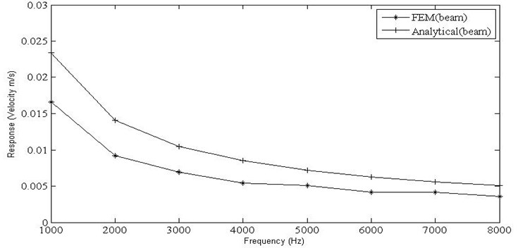
The results for velocity responses obtained for horizontal beam with unit force loading against the variation in frequencies for a width of 0.01 m and internal loss factor of 0.04 has been plotted in Fig. 11. In all the cases, the velocity response decreases with increase in the frequencies, as expected. The velocity responses obtained using the finite element method are closer to the responses found using analytical wave approach for beams with increase in the frequency.

Fig. 11Velocity responses for the horizontal beam

The results for velocity responses obtained for horizontal plate with unit force loading against the variation in frequencies for a plate width of 0.9 m and internal loss factor of 0.04 has been plotted in Fig. 12. The trend of the observed curves remains similar to the earlier one; and the velocity responses obtained using analytical wave approach and Free-SEA software are similar with a close match in the values obtained using the finite element method, as the plate theories govern the results for the considered width.

Fig. 12Velocity responses for the horizontal plate

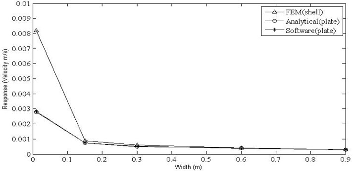
Finally the results for velocity responses obtained for horizontal plate under the action of unit force on it has been plotted in Fig. 13 against the variation in widths of the plate for the value of internal loss factor of 0.04 and a frequency of 8000 Hz. The velocity responses obtained using the analytical wave approach for plates; finite element method and Free-SEA software closely match with each other at larger values of widths. The velocity responses obtained using analytical approach and finite element method for beams agrees well with each other. Similarly the velocity responses obtained by the analytical wave approach for plates and Free-SEA software is underestimated for lower values of widths, whereas the velocity responses obtained using finite element method overestimates the responses at lower widths.

Fig. 13Velocity responses for horizontal plate

5. Conclusions

The CLF values computed by analytical wave approach for beam, plates and the free-sea software are independent of the change in width and damping/internal loss factor. The CLF computed using finite element method increases linearly as the internal loss factor varies from a zero value, followed by a transition region and converges to the values obtained by the analytical wave approach and remains insensitive to changes at higher values of damping. At low values of damping, common for most of the materials, the coupling factors computed by the analytical approach would be overestimated. The coupling factor computed by finite element methods or experimental SEA is expected to be more accurate in this region.

The accuracy of the CLFs and velocity responses computed using the finite element and analytical wave approach for plates/shells is in agreement for larger values of widths, wherein the plate/shell theories are valid. The velocity responses obtained by the analytical wave approach for plates and Free-SEA software is underestimated for lower values of widths, whereas the velocity responses obtained using finite element method overestimates the responses at lower widths. Similarly, the velocity responses obtained using analytical approach and finite element method for beams agree well with each other, but underestimate the responses at larger widths as the beam theory assumptions become invalid.

References

Lyon R. H. Theory and Applications of Statistical Energy Analysis. Second edition, Butterworth-Heinemann, Boston, 1995.

Search CrossRef
Lyon R. H. Statistical Energy Analysis of Dynamical Systems. Massachusetts Institute of Technology, 1975.

Search CrossRef
Bies D. A., Hamid S. Insitu determination of coupling loss factors by the power injection method. Journal of Sound and Vibration, Vol. 70, 1980, p. 187-204.

Search CrossRef
Fahy F. J. An alternative to the SEA coupling loss factor: rationale and method for experimental determination. Journal of Sound and Vibration, Vol. 214, Issue 2, 1998, p. 261-267.

Search CrossRef
Shankar K., Keane A. J. Vibrational energy flow analysis using a substructure approach: the application of receptance theory to FEA and SEA. Journal of Sound and Vibration, Vol. 201, Issue 4, 1997, p. 491-513.

Search CrossRef
Hoplins C. Experimental statistical energy analysis of coupled plates with wave conversion at junction. Journal of Sound and Vibration, Vol. 322, 2009, p. 155-166.

Search CrossRef
Yap F. F., Woodhouse J. Investigation of damping effects on statistical energy analysis of coupled structures. Journal of Sound and Vibration, Vol. 197, Issue 3, 1996, p. 351-371.

Search CrossRef
Norton M. P. Fundamentals of Noise and Vibration Analysis for Engineers. Cambridge University Press, Cambridge, 1989.

Search CrossRef
Hodges C. H., Nash P., Woodhouse J. Measurement of coupling loss factors by matrix fitting an investigation of numerical procedures. Applied Acoustics, Vol. 22, 1987, p. 47-69.

Search CrossRef
Le Bot A., Cotoni V. Validity diagrams of statistical energy analysis. Journal of Sound and Vibration, Vol. 329, 2010, p. 221-235.

Search CrossRef
Rabbiolo G., Bernhard R. J., Milner F. A. Definition of a high-frequency threshold for plates and acoustical spaces. Journal of Sound and Vibration, Vol. 277, Issue 204, p. 647-667.

Search CrossRef
Shankar K., Keane A. J. A study of the vibrational energies of two coupled beams by finite element and green function (receptance) methods. Journal of Sound and Vibration, Vol. 181, Issue 5, 1995, p. 801-838.

Search CrossRef
ANSYS 10.0 Version manual.

Search CrossRef
Keane A. J., W. G. Price SEA – an Overview, with Applications in Structural Dynamics. Cambridge University Press, 2005.

Search CrossRef
Cremer L., Heckl M., Ungar E. E. Structure-Borne Sound. Springer-Verlag, New York, 1973.

Search CrossRef
Clarkson B. L., Pope R. J. Experimental determination of vibration parameters required in the statistical energy analysis method. ASME, Vol. 105, 1983, p. 337-344.

Search CrossRef
Hopkins C. Sound Insulation. 1st Edition, Butterworth-Heinemann, Boston, 2007.

Search CrossRef
Wei G. W., Zhao Y. B., Xiang Y. A novel approach for the analysis of high frequency vibrations. Journal of Sound and Vibration, Vol. 257, Issue 2, 2002, p. 207-246.

Search CrossRef
Clarkson B. L. The derivation of modal densities of structures from point impedances. Journal of Sound and Vibration, Vol. 77, Issue 4, 1981, p. 583-584.

Search CrossRef
Wijker J. Random Vibrations in Spacecraft Design. Springer Publication, 2009.

Search CrossRef

About this article

Received

13 August 2013

Accepted

05 November 2013

Published

31 December 2013

Keywords

statistical energy analysis

equipartition of energy

finite element method

spatial averaging

This is an open access article distributed under the Creative Commons Attribution License, which permits unrestricted use, distribution, and reproduction in any medium, provided the original work is properly cited.