Abstract
This study presents a novel numerical algorithm based on an active control approach to reduce the earthquake responses of a smart building structural system. The proposed control algorithm is a synthesis of the adaptive input estimation method (AIEM) and linear quadratic Gaussian (LQG) controller. An unknown system input can be estimated by the AIEM while the LQG controller offers optimal control forces to suppress seismic vibration. The proposed control technique was evaluated for a smart building structural system under seismic vibration on line optimal control problem. The numerical simulation results show that the proposed method has more robust active vibration control performance than the conventional LQG method.
1. Introduction
Civil structures are exposed to dynamic loads from several sources such as earthquake ground motion, hurricanes, tornados, severe tsunamis, moving vehicles and rotating machinery. Many recent earthquake disasters have occurred around the world during the last twenty years, causing innumerable losses in human life and property. Earthquake resistant design is quite challenging due to the inherent constraints of economics, demand for extreme reliability and the considerable uncertainty in structure design. Under such conditions that the control concept be applied to civil structures is a serious consideration.
To protect the safety and service ability of structures the active structural control theory has rapidly developed during the two last decades. Yang (1975) applied the optimal control theorem to control vibrations in civil engineering structures under stochastic dynamic loads such as earthquakes and wind loads [1]. Chung et al. (1987) presented an experimental study of active control for single degree of freedom and multiple degree of freedom seismic structures using tendons through an optimal closed-loop control scheme [2]. Xu et al. (1999) applied the dominant internal model approach to implement the predictive control of structural responses to external excitations [3]. Akhiev et al. (2002) used the multipoint performance index for the vibration suppression of earthquake-excited structures [4]. Active vibration reduction under harmonic excitation is achieved using both strain and displacement feedback control [5]. Pnevmatikos et al. (2009) presented a control algorithm for seismic protection of building structures based on the theory of variable structural control [6]. Jin et al. (2010) presented the optimal design of vibration control system for smart structures using semi-analytical method via the optimization of geometric parameters [7]. Madhekar et al. (2010) studied the performance of variable dampers for seismic protection of the benchmark highway bridge under six real earthquake ground motions [8]. Chen et al. (2010) presented a general approach in the time domain for integrating vibration control and health monitoring of a building structure to accommodate various types of control devices and on-line damage detection [9]. In all of the above-mentioned methods, the control force is obtained using the displacement and velocity feedback responses of the structures. In other words, the external load influence is not considered in the optimal controller design because the external load disturbances are immeasurable or inestimable in the control force calculation. Therefore, the structure acceleration should be controlled simultaneously. The first objective in this study is to develop a novel method for the required control forces in a complete active control system.
This study first investigates active control technique application to reduce a smart building structural system subjected to earthquake excitations. The active control technique is a synthesis algorithm of the AIEM and LQG controller. The input estimation method has been successfully used to inversely solve 1-D and 2-D heat conduction problems [10, 11] and identify input forces for structural systems [12-14]. The AIEM is frequently employed in structural dynamic problems [15]. An inverse estimation method was proposed for the input forces of a fixed beam structural system [16]. The input estimation method uses the recursive form to process the measurement data. As opposed to the batch process using the recursive form is an on-line process that has higher efficiency. The feasibility of the proposed method is verified using active vibration control numerical simulations of a smart building structural system. The AIEM first can estimate on-line dynamic loads. An active LQG controller can apply the same inverse control forces on a structural system. The control results show that the proposed method is more effective in suppressing vibration in a smart building structural system than the conventional LQG method.
2. Problem formulation
To illustrate the practicability and precision of the presented approach in controlling the unknown earthquake ground motion accelerations, the numerical simulations of the 3D dynamic structure are investigated in this study. As shown in Fig. 1, the dynamic structure is modeled as a lumped mass structure system undergoing the earthquake accelerations. The base was excited by the ground motion accelerations of the 9/21 Chi-Chi earthquake in Taiwan and the EI CENTRO earthquake acceleration. This study proposed the AIEM can estimate on-line the ground motion accelerations; meanwhile, it can be feed backed into the LQG controller which can apply the same inverse control forces effectively in suppressing vibration for a smart building structural system.
Fig. 1A skeleton diagram mathematics model of the 3D building structure
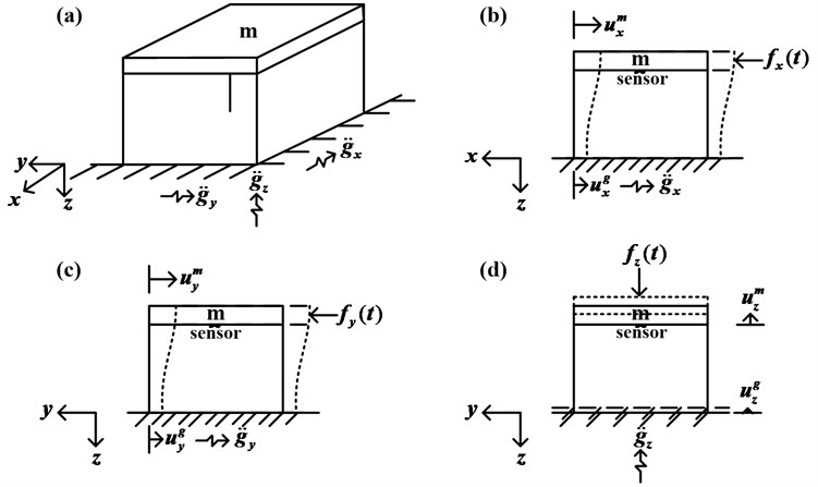
The relative displacement between the lumped mass and ground is represented as the variable , where . The movement equations for the structure system are shown in the following equations:
where represents the damping ratio. is the natural frequency. is the ground motion acceleration. is the control force vector. is the relative velocity. is the relative acceleration, and the subscripts , and represent the weights in every coordinate axis.
In converting the equations of motion to the state variable notation, let and The continuous time state equation and measurement equation of the system can be written as follows:
where
.
is constant matrix. is the state vector. is the vector of control force inputs. and are the coefficient vectors of and , respectively. is the observation vector and is the measurement matrix.
Noise turbulence always exists in the practical environment. This is the reason that any of the physical systems contains two portions. The first is the deterministic portion and the second is the random portion, which is distributed around the deterministic portion. Equations (4) and (5) do not take the noise turbulence into account. In order to construct a statistical model of the system state characteristics, a noise disturbance term that can reflect the state characteristics will need to be added into these two equations. Up to now one of the random noise disturbances that can be completely resolved is the Gaussian white noise, which has been statistically illustrated in full using the probability distribution function and the probability density function. Practically any function corresponding to the functions mentioned above has the same effect. The characteristic function of the random variable is one example. Two most important characteristic values are the mean and variance which represent the statistic properties of the random process [17]. Taking the above consideration into account, the continuous-time state equation can be sampled with the sampling interval , to obtain the discrete-time statistic model of the state equation [18] shown as the following:
where:
is the state vector. is the state transition matrix. is the input matrix. is the sampling interval. is the sequence of deterministic acceleration inputs, is the control array and is the processing error vector, which is assumed as Gaussian white noise. Note that and . are the discrete-time processing noise covariance matrix. is the Kronecker delta function. When describing the structural system active characteristics the additional term can be used to present the uncertainty in a numerical manner. The uncertainty could be the random disturbance, the uncertain parameters, or the error due to numerical model over simplification.
Generally speaking the system state can be determined by measuring the system output. The measurement usually has a certain relationship with the system output. However there is also the noise issue with the measurement. As a result, the discrete-time measurement vector statistical model can be presented as the following:
where:
is the observation vector. represents the measurement noise vector and is assumed to be Gaussian white noise with zero mean and the variance where is the discrete-time measurement noise covariance matrix. is the measurement matrix.
3. AIEM combined LQG control technique design
For standard linear quadratic Gaussian problems the system under control is assumed to be described using the stochastic discrete-time state space equation as below [19]:
where is zero-mean white noise with variances . In general the input forces sequences are neglected or assumed to be zeros in conventional LQG controller design. From Eq. (8) the conventional LQG control methodology for a system without input forces term is obvious. That is to say, the system, Eq. (8) is not satisfactory to model most dynamic structures because there usually are external exciting forces. Therefore we considered the case where the input forces were not zeros, i.e. Eq. (4) and (5). However the conventional LQG control methodology is not applicable for structures without neglecting the input disturbance forces, because the entire input dynamic loads histories are not known a priori.
The conventional LQG controller has a specific level of interference suppression. It is weak in maintaining high performance in the suppression of external loads, which are complex and arbitrary style disturbances. In other words, in Eq. (4), if a time-varying load exists, the optimal control method combining the Kalman filter and the LQG regulator will not be able to obtain the optimal control forces. To resolve this situation this study proposes combining the AIEM with the LQG control technique for smart building structural system active vibration control. The AIEM can estimate the unknown dynamic inputs while the active LQG controller can apply the same inverse control forces on the structural system.
The AIEM is composed of a Kalman filter without the input term and the adaptive weighting recursive least square algorithm. The detailed formulation of this technique can be found in the research of Tuan et al. [20]. The Kalman filter optimal estimation equations are as follows.
The optimal estimate of the state is:
The bias innovation produced by the measurement noise and input disturbance is expressed by:
The Kalman gain is:
The residual covariance is :
The prediction error covariance matrix is:
The recursive least square estimator equations are as follows.
The sensitivity matrices are and
The correction gain is expressed as:
The error covariance of the input estimation process is:
The estimated earth motion acceleration is:
According to Eq. (10) the innovation with variation is caused by the measurement noise and the unknown input noise. If a large input variation exists can be set as the abnormal or long-tail distribution. Huber used the least favorable probability density function (PDF) to describe the residual in a flexible manner which is either normal or abnormal. In this study Here the least favorable PDF is defined as follows:
where is the adjustable constant to adjust the estimator robustness. According to Eq. (19), if , is a normal distribution; if , is a long-tail distribution. By adopting the double-exponent density function to describe the possible abnormal samples and lower the influence of the estimation weight the robustness can be obtained. Therefore  can be regarded as a threshold, which is the function , which is a reasonable threshold. is the standard deviation of the measurement error. In Eqs. (16-17) is a weighting factor using the adaptive weighting function in this study formulated in (Tuan, et al. 1998) [11]. That is:
Fig. 2Flowchart of the AIEM estimator
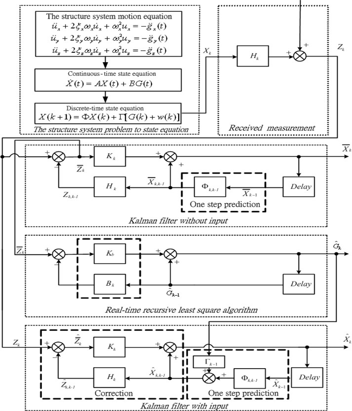
The weighting factor as shown in Eq. (20) can be adjusted according to the measurement noise and input bias. In industrial applications the standard deviation is assumed as a constant value. The magnitude of the weighting factor is determined according to the bias innovation modulus The unknown input prompt variation will cause the large bias innovation modulus. In the meantime the smaller weighting factor is obtained when the bias innovation modulus is larger. Therefore the estimator accelerates the tracking speed and produces larger vibration in the estimation process. Conversely, the smaller unknown input variation causes a smaller bias innovation modulus. Meanwhile a larger weighting factor is obtained according to the smaller bias innovation modulus. A flow chart of the AIEM estimator is given in Fig. 2.
In the LQG optimal control method estimation portion by substituting of Eq. (18) for and substituting the control input in Eq. (9), the optimal state estimation equation can be rewritten as:
The performance index is defined as:
where , and are all symmetrical weighting matrices. The optimal feedback control force vector can be obtained by using the separation theorem [21]:
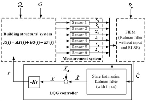
Fig. 3Flowchart of the AIEM combined with the LQG
Here the regular gain is given by:
where is the discrete-time Ricatti equation solution. The Ricatti equation is shown below:
According to Eq. (25) can be obtained by inversely calculating from to The method combining AIEM and the LQG active controller is presented using the AIEM to estimate and combining Eq. (21) to obtain the optimal state estimate which can be further substituted in Eq. (23). The combination of AIEM and the LQG controller is illustrated in Fig. 3.
4. Results and discussion
To demonstrate the accuracy and efficiency of the proposed controller design two smart building structural system numerical simulation cases are investigated. The building structure mass 3450.6 kg. It is assumed that the building is a symmetrical structure with the lateral stiffness of a single column (N/m) and axial stiffness (N/m). The material data and dimensions of the column are shown in Table 1.
Table 1The material data and dimensions of the column
Elastic modulus, | 200 GPa |
Length, | 3.5 m |
Cross-sectional area, | 0.16 m2 |
Moment of inertia, | (0.4)4⁄12 m4 |
Damping coefficient, | 2937 Ns/m |
The active reaction of a smart building structural system under ground motion acceleration inputs must be determined in the first stage. This method is composed of the adaptive input estimation method (AIEM) and linear quadratic Gaussian (LQG) controller. The initial conditions and other parameters of the simulation are shown as follows: , , . is set as a zero matrix. The sampling interval and the total simulation time . The weighting factor is an adaptive weighting function. The process noise and measurement noise are both considered in the simulation process. The process noise covariance matrix , where . The measurement noise covariance matrix , where . is the standard deviation of noise.
4.1. Example 1. The 921 Chi-Chi earthquake
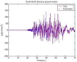
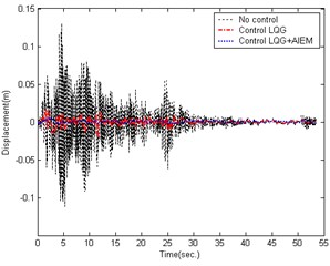
The ground motion accelerations of the 921 Chi-Chi earthquake in Taiwan were measured from the seismological station (TCU056) at Li-Ming Elementary School. The unknown ground motion accelerations can also be estimated from the roof displacements of the smart building structural system. Fig. 4 shows the estimated smart building structural system result to earth motion acceleration in the East-West direction. The estimated South-North direction result is shown in Fig. 5. The time histories of the responses for a smart building structural system with and without control are shown in Figs. 6-7.
Fig. 4The estimated building structure results caused by the 921 Chi-Chi Earthquake in the East-West direction
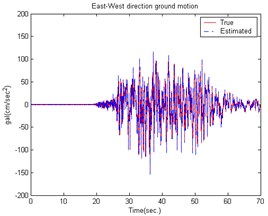
Fig. 5The estimated building structure results caused by the 921 Chi-Chi Earthquake in the South-North direction
The conventional LQG controller has an issue that the unknown input cannot be obtained and the control reaction is slower. The AIEM estimates the unknown input on-line and combined with the LQG controller (which computes the optimal control force) can be used to obtain better results.
Fig. 6Comparison of building displacement control (East-West direction) caused by the 921 Chi-Chi Earthquake
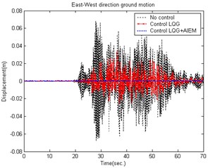
Fig. 7Comparison of building displacement control (South-North direction) caused by the 921 Chi-Chi Earthquake
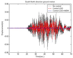
Fig. 8The estimated building structure results caused by the EI CENTRO Earthquake in the East-West direction
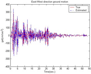
Fig. 9The estimated building structure results caused by the EI CENTRO Earthquake in the South-North direction
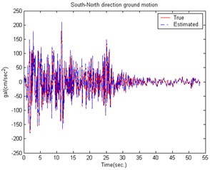
Fig. 10Comparison of building displacement control (East-West direction) caused by the EI CENTRO Earthquake
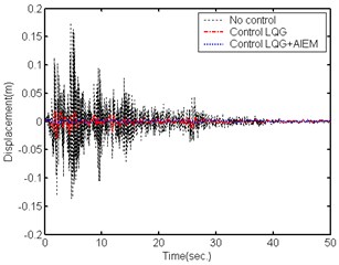
Fig. 11Comparison of building displacement control (South-North direction) caused by the EI CENTRO Earthquake
4.2. Example 2. The EI CENTRO earthquake
The effectiveness of the proposed active control technique was further demonstrated by the ground motion acceleration estimation of the EI CENTRO earthquake (1940). Fig. 8 shows the estimated result for a smart building structural system to earth motion acceleration in the East-West direction. The estimated South-North direction result is shown in Fig. 9. The estimation results show that the estimator tracking performance is good enough and suitable for reducing the noise effect. Figs. 10-11 show a comparison of the building roof displacements with and without control using distinct controllers under the EI CENTRO earthquake. The proposed controller has good control performance due to the larger control forces. The simulation results demonstrate that the proposed control method successfully reduces the smart building structural system responses when subjected to seismic excitation.
5. Conclusions
This study proposed an active control technique for active ground motion acceleration control in a smart building structural system. The combination of the excellent AIEM and LQG controller produced a feasible control approach to reduce the vibration. Because this active control technique requires external forces information, the AIEM is proposed for on-line excitation estimation. The developed controller demonstrated excellent performance by solving the earthquake excitation structure vibration suppression problem. The results demonstrate that the proposed technique is more effective in reducing seismic responses than the conventional LQG controller. Future work is being conducted to extend this application to a nonlinear structural system.
References
-
Akhiev S. S., Aldemir U., Bakioglu M. Multipoint instantaneous optimal control of structures. Computers and Structures, Vol. 80, 2002, p. 909-917.
-
Bogler P. L. Tracking a maneuvering target using input estimation. IEEE Transactions on Aerospace and Electronic Systems, Vol. 23, Issue 3, 1987, p. 298-310.
-
Chan Y. T., Hu A. G. C., Plant J. B. A Kalman filter based tracking scheme with input estimation. IEEE Transactions on Aerospace and Electronic Systems, Vol. 15, Issue 2, 1979, p. 237-244.
-
Chen B., Xu Y. L., Zhao X. Integrated vibration control and health monitoring of building structures: a time-domain approach. Smart Structures and Systems, Vol. 6, Issue 7, 2010, p. 811-833.
-
Chen T. C., Lee M. H. Inverse active wind load inputs estimation of the multilayer shearing stress structure. Wind and Struct., An Int. J., Vol. 11, Issue 1, 2008, p. 19-33.
-
Chung L. L., Reinhorn A. M., Soong T. T. Experiments on active control of seismic structures. J. of Eng. Mech., ASCE, Vol. 114, Issue 2, 1988, p. 241-256.
-
Deng S., Heh T. Y. The study of structural system dynamic problems by recursive estimation method. Int. J. Adv. Manuf. Technol., Vol. 30, 2006, p. 195-202.
-
Jin Z., Yang Y., Soh C. K. Semi-analytical solutions for optimal distributions of sensors and actuators in smart structure vibration control. Smart Struct. and Sys., Vol. 6, Issue 7, 2010, p. 767-792.
-
Kwakernaak H., Sivan R. Linear Optimal Control System. Wiley, New York, 1972.
-
Lee M. H., Chen T. C. Blast load input estimation of the medium girder bridge using inverse method. Defense Sci. J., Vol. 58, Issue 1, 2008, p. 46-56.
-
Lee M. H., Chen T. C. Estimation of input force on the plate structure by the inverse method. Struct. Eng. and Mech., An Int. J., Vol. 31, Issue 1, 2010, p. 1-14.
-
Lee M. H. Estimation of structure system input force using the inverse fuzzy estimator. Struct. Eng. and Mech., An Int. J., Vol. 37, Issue 4, 2011, p. 351-366.
-
Lewis F. L., Syrmos V. L. Optimal Control. Wiley, New York, 1972.
-
Madhekar S. N., Jangid R. S. Seismic response control of benchmark highway bridge using variable dampers. Smart Struct. and Sys., Vol. 6, Issue 8, 2010, p. 953-974.
-
Malgaca L., Karagulle H. Simulation and experimental analysis of active vibration control of smart beams under harmonic excitation. Smart Struct. and Sys., Vol. 5, Issue 1, 2009, p. 55-68.
-
Pnevmatikos N. G., Gantes C. J. Sliding mode control for structures based on the frequency content of the earthquake loading. Smart Struct. and Sys., Vol. 5, Issue 3, 2009, p. 209-221.
-
Tuan P. C., Fong L. W., Huang W. T. Analysis of on-line inverse heat conduction problems. J. of Chung Cheng Institute of Technology, Vol. 25, Issue 1, 1996, p. 59-73.
-
Tuan P. C., Lee S. C., Hou W. T. An efficient on-line thermal input estimation method using Kalman filter and recursive least square algorithm. Inverse Problem Eng., Vol. 5, 1997, p. 309-333.
-
Tuan P. C., Hou W. T. Adaptive robust weighting input estimation method for the 1-D inverse heat conduction problem. Numeral Heat Transfer, Vol. 34, 1998, p. 439-456.
-
Xu N. S., Yang Z. H. Predictive structural control based on dominant internal model approach. Automatica, Vol. 35, 1999, p. 59-67.
-
Yang J. N. Application of optimal control theory to civil engineeringstructures. J. Eng. Mech. Div., Vol. 101, Issue 6, 1975, p. 819-838.
About this article
This study was partially supported by the National Science Council in Taiwan, R. O. C. through Grant NSC 100-2221-E-145-002.
