Verification of bee algorithm based path planning for a 6DOF manipulator using ADAMS

Masajedi, Pedram; Heidari Shirazi, Kourosh; Ghanbarzadeh, Afshin

Journal of Vibroengineering

Browse Journal

Submit article

Published: 30 June 2013

Check for updates

Verification of bee algorithm based path planning for a 6DOF manipulator using ADAMS

Pedram Masajedi¹

Kourosh Heidari Shirazi²

Afshin Ghanbarzadeh³

^{1, 2, 3}Shahid Chamran University of Ahvaz, Department of Mechanical Engineering, Ahvaz, Iran

Cite the article Download PDF

Downloads 1268

Abstract

In this article the end effector displacement control for a manipulator robot with 6 rotational joints on a predetermined 3-dimensional trajectory is investigated. Since for any end effector position there are more than a single set of answers, regarding to robot parts orientation, finding a method which gives the designer all existing states will lead to more freedom of action. Hence two different methods were applied to solve robot inverse kinematic issue. In the first method ADAMS software was considered, which is a well-known software in the field of solving inverse kinematic problems, and after that BA algorithm is used as an intelligent method. This method is one of the fastest and most efficient methods among all existing ones for solving non-linear problems. Hence problem of inverse kinematic solution is transformed into an affair of optimization. Comparison of results obtained by both models indicates the reasonable performance of BA because of its capability in providing the answers from all existing states along with the privilege of no need to 3D modeling.

1. Introduction

Conducted researches in the field of robotics include a wide range of theoretical and practical topics like motion planning [1], intelligent control [2, 3], and motion control on predetermined 3-dimensional trajectories [4]. Trajectory design for robot arms is usually performed in Cartesian space and determination of robot joint movements by having the location and orientation of end effector is called robot inverse kinematics.

In robotics, end effector is a tool at the end of robot arm which is designed for interactions with external environment. Its exact nature is dependent on robot functions. In serial robots, end effector is defined as the robot ultimate link which has the duty of attaching robot to the target object. To give a more precise definition, end effector is a member of robot that interacts with environment.

There are different methods for solving inverse kinematic problem including algebraic, geometrical, and trial and error methods, which are both time consuming and difficult to be solved numerically [5, 6]. In recent years there have been numerous efforts to use new methods in revers kinematics solutions. Koker et al [7] considered a multi-layer neural network design for a robot with 3 degrees of freedom in 2004. Durmus et al [8] solved inverse kinematic for a robot with 6 degrees of freedom using BA algorithm in 2011.

The most important subject in using new problem solving methods is that given Denavit-Hartenberg parameters, without having 3D designs, it is possible to compute desired angles of joints, which makes design process much simpler.

2. Inverse kinematic

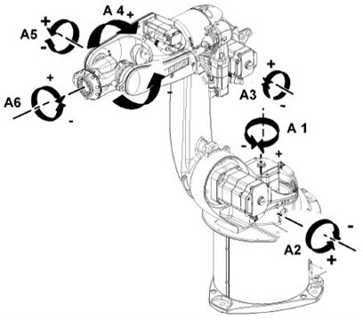
Fig. 1 shows the KOKA KR16 robot which is studied in this article.

For a robot with $n$ degrees of freedom, relation between joints is given by (1):

1

x (t) = f (θ (t)),

where $x (t)$ is the position of end effector, $θ (t)$ is the vector of robot joints angles, and $f$ is a nonlinear continuous function that relates joint variables to work environment coordination. This equation has only a unique answer solvable by analytical methods [9]. In the other hand, it is possible to solve the inverse kinematic problem by solution of the following equation:

2

θ (t) = f^{- 1} (x (t)) .

Unlike direct kinematics, this equation does not have a unique answer. In order to solve inverse kinematic, Denavit-Hartenberg system needs to be defined on robot firstly.

Fig. 1KR16 robot arms degrees of freedom

3. Denavit-Hartenberg system

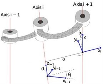
In order to express the relative motion of end effector from fixed joint, a matrix needs to be defined which includes relative rotation and replacement of determined coordinate system from earth coordinate system. For this purpose, Denavit-Hartenberg system is considered for each joint. Fig. 2 illustrates the orientation of different coordinate systems for each joint and also demonstrates how the values applied in kinematics table are determined.

Fig. 2Definition of Denavit-Hartenberg parameters

According to definition, a rotational matrix that describes each joint relative to the previous joint is given by (3):

3

{}^{n - 1}{T_{n}} = [\begin{matrix} c o s θ_{n} & - s i n θ_{n} c o s α_{n} & s i n θ_{n} s i n α_{n} & a_{n} c o s θ_{n} \\ s i n θ_{n} & c o s θ_{n} c o s α_{n} & - c o s θ_{n} s i n α_{n} & a_{n} s i n θ_{n} \\ 0 & s i n α_{n} & c o s α_{n} & d_{n} \\ 0 & 0 & 0 & 1 \end{matrix}] .

And finally, the matrix determining orientation and location of end effector is derived from calculated matrix of (3) for each joint:

4

{{}^{6}T}_{0} = {{}^{0}T}_{1} {{}^{1}T}_{2} {{}^{2}T}_{3} {{}^{3}T}_{4} {{}^{4}T}_{5} {{}^{5}T}_{6} = [\begin{matrix} n_{x} & s_{x} & a_{x} & p_{x} \\ n_{y} & s_{y} & a_{y} & p_{y} \\ n_{z} & s_{z} & a_{z} & p_{z} \\ 0 & 0 & 0 & 1 \end{matrix}] .

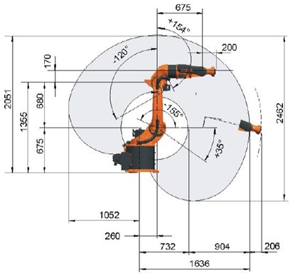
Fig. 3. illustrates motion restrictions for KOKA KR16 along with specifications.

Fig. 3Geometric characteristics of KR16

4. Analytical solution

According to definition, a robot arm will have redundancy if for an end effector state there is more than a set of answers for joint angles [10]. For a specific position of end effector, there are 8 possible states presented in Fig. 4.

Fig. 4Possible solution for KR16 robot inverse kinematic problem

4.1. Joint 1

Joint number 1 is considered for analytical solution of robot inverse kinematic problem and all possible states will be calculated for it; this procedure will be continued through all joints to number 6.

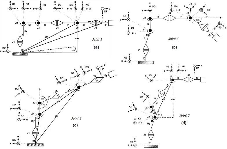
According to Fig. 5(a), the position vector ${\vec{p}}_{04}$ will be:

5

{\vec{p}}_{04} = \vec{p} - {\vec{p}}_{46} = \vec{p} - (l_{5} + l_{F}) \vec{n} .

Fig. 5Joints orientation

Thus $θ$ and $θ + π$ are two possible solutions for joint number 1 angle that could be calculated from (6):

6

\{\begin{array}{l} θ_{1,1} = θ_{1,2} = θ_{1,3} = θ_{1,4} = arctan 2 (- p_{04, z}, p_{04, x}), \\ θ_{1,5} = θ_{1,6} = θ_{1,7} = θ_{1,8} = arctan 2 (- p_{04, z}, p_{04, x}) + π . \end{array}

4.2. Joint 3

Via the knowledge of $p_{14}$ value, $ϕ$ would be determined which in turn leads to joint angle $θ_{3}$ . As shown in Fig. 5(c), the angular state of joint number 4 influences the orientation of frame $K_{4}$ and has no effect on its location; hence we could calculate vector $p_{14}$ from (7):

7

{\vec{p}}_{14} = {\vec{p}}_{04} - {\vec{p}}_{01} .

Now the angle of $ϕ$ could be calculated from (8):

8

ϕ = \arccos (\frac{l_{2}^{2} + {(l_{3} + l_{4})}^{2} - | p_{14} |^{2}}{2 l_{2} (l_{3} + l_{4})}) .

Finally, knowledge of $ϕ$ offers eight possible solutions for $θ_{3}$ :

9

θ_{3,1} = θ_{3,2} = π - ϕ, θ_{3,3} = θ_{3,4} = π + ϕ, θ_{3,5} = θ_{3,6} = - (π - ϕ),

θ_{3,7} = θ_{3,8} = - (π + ϕ) .

4.3. Joint 2

As shown in Fig. 5(d), angle $θ_{2}$ could be calculated by $β_{1}$ , $β_{2}$ . Since vector $p_{14}$ has only two components of $x$ and $z$ , for a simpler calculation of $β_{1}$ , vector $p_{14}$ could be transferred from coordinate system 0 to 1 by (10):

10

{{}^{0}T}_{1} = {{}^{0}D}_{1} (α_{0}, a_{0}, d_{1}, θ_{1}) = (\begin{matrix} {{}^{0}R}_{1} & \vec{p} \\ {\vec{0}}^{T} & 1 \end{matrix}), {}^{1}{\vec{p}}_{14} = {({{}^{0}R}_{1})}^{- 1} {\vec{p}}_{14} .

Hence values of $β_{1}$ and $β_{2}$ could be calculated from (11):

11

β_{1} = a r c t a n ({}^{1}{\vec{p}}_{14, x}, {}^{1}{\vec{p}}_{14, z}), β_{2} = a r c c o s (\frac{l_{2}^{2} + |p_{14}| - {(l_{3} + l_{4})}^{2}}{2 l_{2} |p_{14}|}) .

And finally four $θ_{2}$ values will come from (12):

12

θ_{2,1} = θ_{2,2} = - (β_{1} + β_{2}), θ_{2,3} = θ_{2,4} = - (β_{1} - β_{2}), θ_{2,5} = θ_{2,6} = (β_{1} + β_{2}),

θ_{2,7} = θ_{2,8} = (β_{1} - β_{2}) .

4.4. Joint 5

Angle of joint number 5 is derived from internal multiplication of vectors $n$ and $z_{4}$ :

13

z_{4} ∙ n = |z_{4}| ∙ | n | ∙ c o s (θ_{5}) \Rightarrow θ_{5} = a r c c o s (z_{4}, n) .

Vector $z_{4}$ orientation could be derived from ${{}^{0}R}_{4}$ rotation. Angle $θ_{4}$ has no effect on $z_{4}$ location, so value of $θ_{4}$ is assumed zero. Using $θ_{1}$ , $θ_{2}$ and $θ_{3}$ from previous calculations, ${{}^{0}T}_{4}$ could be calculated:

14

{{}^{0}T}_{4} = {{}^{0}D}_{1} (α_{0}, a_{0}, θ_{1}, d_{1}) {{}^{1}D}_{2} (α_{1}, a_{1}, θ_{2}, d_{2}) {{}^{2}D}_{3} (α_{2}, a_{2}, θ_{3}, d_{3}) {{}^{3}D}_{4} (α_{3}, a_{3}, θ_{4}, d_{4}) .

Equation (15) for ${{}^{0}T}_{4}$ is obtained by expansion of (14):

15

{{}^{0}T}_{4} = (\begin{matrix} {{}^{0}R}_{4} & \vec{p} \\ 0 & 1 \end{matrix}), {{}^{0}R}_{4} = (x_{4}, y_{4}, z_{4}) = {{}^{0}R}_{1} (θ_{1}) {{}^{1}R}_{2} (θ_{2}) {{}^{2}R}_{3} (θ_{3}) {{}^{3}R}_{4} (θ_{4}) .

Having vector $z_{4}$ from matrix above, $θ_{5}$ could be calculated from (16):

16

\{\begin{matrix} θ_{5,1} = θ_{5,2} = a r c c o s (z_{4 A} n), θ_{5,3} = θ_{5,4} = - a r c c o s (z_{4 A} n), \\ θ_{5,5} = θ_{5,6} = a r c c o s (z_{4 B} n), θ_{5,7} = θ_{5,8} = - a r c c o s (z_{4 B} n) . \end{matrix}

4.5. Joints 4 and 6

Total rotation matrix could be obtained from equation (17):

17

{{}^{0}R}_{7} = {{}^{0}R}_{4} {{}^{4}R}_{7} \to {{}^{4}R}_{7} = {({{}^{0}R}_{4})}^{- 1} ({{}^{0}R}_{7}) = {{}^{0}R}_{4} {{}^{0}R}_{7}

\Rightarrow {({{}^{0}R}_{4})}^{T} {{}^{0}R}_{4} = I \to {{}^{0}R}_{4} = {({{}^{0}R}_{4})}^{- 1} .

Rotation matrix ${{}^{4}R}_{7}$ could be obtained from 3 rotations below:

18

{{}^{4}R}_{7} = R o t_{z} (θ_{4}) R o t_{y} (θ_{5}) R o t_{z} (θ_{6}) \Rightarrow {{}^{4}R}_{7} = {({{}^{0}R}_{4})}^{T} {{}^{0}R}_{7},

{{}^{4}R}_{7} = (\begin{matrix} c θ_{4} c θ_{5} c θ_{6} - s θ_{4} s θ_{6} & - c θ_{4} c θ_{5} s θ_{6} - s θ_{4} c θ_{6} & c θ_{4} s θ_{5} \\ s θ_{4} c θ_{5} c θ_{6} + c θ_{4} s θ_{6} & - s θ_{4} c θ_{5} s θ_{6} - c θ_{4} c θ_{6} & s θ_{4} s θ_{5} \\ - s θ_{5} c θ_{6} & s θ_{5} s θ_{6} & c θ_{5} \end{matrix}) .

In order to obtain all possible positions, two matrices below should be calculated:

19

{{}^{4}R}_{7, A} = {({{}^{0}R}_{4, A})}^{T} {{}^{0}R}_{7}, {{}^{4}R}_{7, B} = {({{}^{0}R}_{4, B})}^{T} {{}^{0}R}_{7} .

Considering $t a n (α) = s i n (α) {c o s}^{- 1} (α)$ , angle $θ_{4}$ could be calculated from $r_{23}, r_{13}$ and rotation matrix ${{}^{4}R}_{7}$ :

20

θ_{4} = atan 2 (\pm r_{23}, \pm r_{13}) .

So all possible states for $θ_{4}$ will be:

21

\{\begin{matrix} θ_{4,1} = θ_{4,6} = atan 2 (r_{23, A}, r_{13, A}), θ_{4,2} = θ_{4,5} = atan 2 (r_{23, A}, r_{13, A}) + π, \\ θ_{4,3} = θ_{4,8} = atan 2 (r_{23, B}, r_{13, B}), θ_{4,4} = θ_{4,7} = atan 2 (r_{23, B}, r_{13, B}) + π . \end{matrix}

In a similar case, all possible values of $θ_{6}$ could be calculated from (22):

22

\{\begin{matrix} θ_{6,1} = θ_{6,5} = atan 2 (- r_{32, A}, r_{31, A}), θ_{6,2} = θ_{6,6} = atan 2 (- r_{32, A}, r_{31, A}) + π, \\ θ_{6,3} = θ_{6,7} = atan 2 (- r_{32, B}, r_{31, B}), θ_{6,4} = θ_{6,8} = atan 2 (- r_{32, B}, r_{31, B}) + π . \end{matrix}

5. Model of position error

It has been reported in the literature that the gear train errors, the errors due to structural deformations, and the errors due to the geometric parameters of the model can be represented by a cyclic function of the joint angles. Based on this, we assume that the positioning errors change with the joint positions, i.e., $Δ p = f (θ_{i})$ . Another assumption which is made is that the locus of positioning errors for selected identification configuration is a piecewise continuous random function. It follows that the loci of the Cartesian errors of robot manipulators while following a given trajectory are in the form of bounded and integral functions. If a given function of $p (θ)$ can be approximated with a polynomial $F (θ)$ within the defined interval such that:

23

| p (θ) - F (θ) | \leq ε,

$F (θ)$ can be of any type of polynomials including Fourier polynomials, ordinary polynomials, and the other well-known polynomials of Jacobi, Laguerre and Hermite, and Bessel. In this study Fourier and ordinary polynomials are considered for position error approximation.

It had been demonstrated a long time ago [9] that if $p (θ)$ has a discontinuity at $θ = θ_{0}$ , the polynomial $F (θ)$ will converge at $θ = θ_{0}$ to the arithmetic mean of the values $p (θ_{0} -)$ and $p (θ_{0} +)$ of the function $p (θ)$ obtained as $θ$ approaches $θ_{0}$ from the left and from the right, respectively. This means that the function $p (θ)$ is piece-wise continuous in the interval of $(θ_{0} - δ θ_{0}, θ_{0} + δ θ_{0})$ , where $δ θ_{0}$ is the infinitesimal amount by which it is approached to $θ_{0}$ from the left and from the right.

Drawing the same analogy for an $n$ -jointed manipulator, the error functions of $δ x, δ y, δ z$ are piece continuous at the intervals of $θ_{i} - δ θ_{i} \leq θ_{i} \leq θ_{i} + δ θ_{i}$ for $i =$ 1, …, $n$ . This means that the polynomials converge to the expected error values for every identification configuration of the manipulator given in joint space. With this in mind, the position error in each Cartesian direction can be approximated with a trigonometric or Fourier polynomial of:

24

{(δ x)}_{i} = K_{i} + \sum_{q = 1}^{r} [A_{q} \cos (q θ_{i}) + B_{q} \sin (q θ_{i})],

where ${(δ x)}_{i}$ is the positioning error in the x direction due to the movement of the $i$ th joint only, and $θ_{i}$ is the angular position of the $i$ th joint. For an $n$ -jointed manipulator, Eq. (24) can be rewritten as:

25

{(δ x)}_{i} = \sum_{i = 1}^{n} K_{i} + \sum_{q = 1}^{r} [\sum_{i = 1}^{n} A_{q i} \cos (q θ_{i}) + B_{q i} \sin (q θ_{i})],

where $r$ is the number of harmonics. Similar expressions can be written for the position errors of $δ y, δ z$ . Another alternative polynomial to approximate the error functions with this is to employ an ordinary polynomial of the $k$ th degree, which can be expressed as:

26

{(δ x)}_{i} = Q_{i} + \sum_{j = 1}^{k} (A_{i} θ_{i}^{j}) .

For an $n$ -jointed manipulator, Eq. (26) can be rewritten as:

27

{(δ x)}_{i} = \sum_{i = 1}^{n} Q_{i} + \sum_{j = 1}^{k} [\sum_{i = 1}^{n} (A_{j i} θ_{i}^{j})] .

Again, similar expressions can be rewritten for $δ y, δ z$ in the same way as $δ x$ [11].

6. BA based optimization

The bee algorithm is an optimization algorithm inspired from the natural foraging behavior of honey bees. BA was proposed by Pham et al [12]. The BA algorithm receives the following parameters as its inputs: number of bees $(n)$ , number of sites selected out of n visited sites $(m)$ , number of best sites out of $m$ selected sites $(e)$ , number of bees recruited for each best $e$ sites $(n e)$ , number of bees recruited for the other $(m - e)$ selected sites $(n s)$ , number of scout bees $(s)$ . Under this configuration, we will have:

28

n = e \times n e + (m - e) \times n s + s .

The BA algorithm has three phases: initialization, position updating, and termination.

6.1. Initialization

The algorithm starts with the $n$ bees being placed randomly in the search space. Each bee is initialized as follows: assume that we have a project with $n$ activities. First, a set of $n$ random numbers are generated in the range of [0, 1] for the $n$ activities. Then these numbers and their corresponding activities are sorted in descending order. This project has 6 activities. Hence a 6-dimensional vector is created for a bee and a random number is associated to each dimension. Using this approach, the resultant initial schedule may be infeasible. After initialization, the fitnesses of the sites visited by the bees are evaluated. To evaluate the fitness of a food source we need to generate the schedule from the priority list.

6.2. Position updating

At the start of each cycle of the algorithm a subset of bees that have the highest fitnesses are chosen as “selected bees” and sites visited by them are chosen for neighborhood search. A part of these selected bees (i.e. $e$ of $m$ ) with better fitnesses and $n e$ bees are recruited for each of these bees. The fitness values are used to determine the probability of the bees being selected. The bees can be chosen directly according to the fitnesses associated with the sites they are visiting. The probability $p_{j}$ is defined as a relative fitness of the selected bee $j$ in the set of best $e$ sites:

29

p_{j} = \frac{f i t ({\vec{x}}_{j})}{\sum_{c = 1}^{e} f i t ({\vec{x}}_{c})},

where $f i t ({\vec{x}}_{j})$ is the fitness value of the site visited by bee $j$ which is computed as the way reported in the Section ''fitness evaluation''. Also other $m - e$ selected bees are selected based on (29) and $n s$ bees are recruited around each of them. In BA more bees are assigned to search near to the best $e$ sites. Then, in the next step, the algorithm searches in the neighborhood of the selected sites. Searches in the neighborhood of the best $e$ sites (which represent more promising solutions than other selected bees) recruit more bees to follow them. Together with scouting, this differential recruitment is a key operation of the BA algorithm. The performance of BA method mainly depends on the neighborhood search performed by the recruited bees around the selected bees.

After the neighborhood search, we investigate the performance of each patch. If the neighborhood search fails to bring any improvement of performance after a predetermined number of iterations (called $n i$ ), then the corresponding site should be updated. The $n i$ parameter is determined manually. In this work, the value of $n i$ is set to 3. The abandoned site is replaced by the new one assuming that its position is selected using the following equation:

30

{\vec{x}}_{i, n e w} = {\vec{x}}_{i, o l d} + ω r ({\vec{e}}_{i} - {\vec{x}}_{i, o l d}),

where ${\vec{e}}_{i}$ is the position vector of the interesting elite bee which is selected randomly from the bees with the highest fitnesses, ${\vec{x}}_{i, o l d}$ and ${\vec{x}}_{i, n e w}$ respectively represent the position of the abandoned site and the new one which are selected by the bee $i$ , $r$ is a random variable of uniform distribution in the range of [0, 1] and $ω$ respectively control the importance of the new site which is proposed by the elite bee.

This research aims to identify an inverse kinematics solution that minimizes the fitness function which is the position error expressed as a distance between the robot end effector and the target. The Cartesian coordinate information can be computed using the direct kinematics equations for any new offspring obtained [13, 14]. Next the position error can be easily obtained in metric form by using a three-dimensional (3-D) distance equation between two points in 3-D space. The Euclidean distance formula can be used in the distance computation, as stated in as follows:

31

E r r o r = {(x - x_{d e s i r e d})}^{2} + {(y - y_{d i s i r e d})}^{2} + {(z - z_{d i s i r e d})}^{2} .

The number of scout bees used in optimization with BA is 50, number of best selected patches is 3, number of elite selected patches is 1, number of recruited bees around best selected patches is 4, and patch radius for neighborhood search is selected 0.02.

7. Simulation results

In this section results evaluated by ADAMS and BA will be illustrated. In order to obtain Adams results, the robot is simulated in ADAMS environment and then it has been constrained by the end effector to move on predetermined path. Subsequently corresponding joints variations are measured through the path [15].

To evaluate the BA results, 21 accuracy points are defined as a presumed trajectory to be followed by the end effector and then a set of joint angles will be calculated from (31) according to BA process. By accounting motion limitation of each joint, 8 possible answers are accessible for a specific target [16, 17].

By using interpolation method between driven angles for each joint, related spline could be obtained. Then these splines are assumed as the motor input for each joint in ADAMS. Consequently, end effector movement according to joints input evaluated by BA is compared with predetermined trajectory in order to test its reliability. Fig. 6 shows 2 different sets of joint angles obtained by BA (blue dot) and ADAMS (red line) for the same end effector predetermined trajectory.

Fig. 6Joints variation evaluated by ADAMS and BA

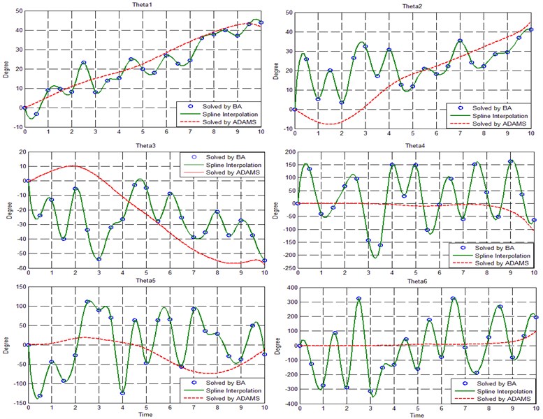
According to Figs. 6, the green curve exhibits calculated joint angles via BA which are connected to each other using 6th order interpolation and in order to move on desired trajectory.

By inserting calculated values for each joint, based on selected accuracy points, and using equations (3) and (4), $p_{x}, p_{y}, p_{z}$ will be evaluated [18, 19]. Fig. 7 shows these amounts (black dot) which are connected to each other using sixth-order interpolation.

In order to study the calculated joint angles more precisely, estimated values through BA (Fig. 6) are imported as motor inputs in ADAMS. Fig. 8 shows that how robot moves in ADAMS environment regarding imported amounts for each joint.

In Fig. 8 green curve shows the difference between traversed trajectory and desired one. As it is depicted in the figure, end effector follows the desired path while created error is close to zero. Undoubtedly, using more accuracy points will increase the precision of tracking [20].

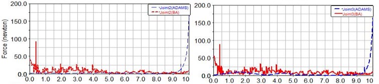
According to Fig. 9, forces tolerated by joints in a situation in which values calculated by ADAMS are used have a more uniform trend, while the magnitudes of these forces are greater than values calculated by BA method.

Fig. 7The end effector trajectory for components X, Y and Z

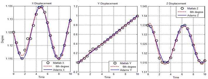
Fig. 8End effector components variation comparison

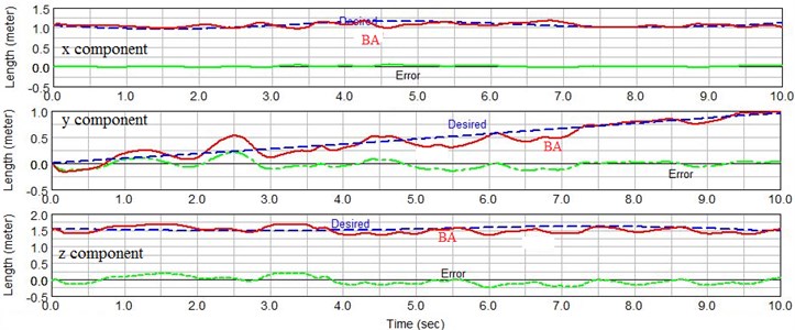
Fig. 9Comparison of force created in joints by ADAMS and BA

a)

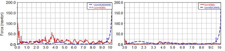
b)

8. Conclusion

In this article inverse kinematic problem is studied for a 6R manipulator robot using ADAMS and BA intelligent optimization method. For this purpose both linear and curved trajectories were considered to evaluate the reliability of mentioned methods.

According to simulation results, ADAMS software exhibited very high precision in predicting joint angles to conduct a robot on a predetermined trajectory, but a precise 3D model will be required and there with, only one of 8 possible states are calculated. To point out some advantages of optimization methods, we could refer to its capability of calculating all possible states for joint angles without a need to 3D simulation of a robot, in a very short time and with a high level of precision. Hence the designer will have more freedom of action in dealing with physical obstacles for a given state by using other states. Also, in order to increase precision, number of accuracy points can be increased so that it satisfies the criteria.

References

Smith K. B., Zheng Y. Optimal path planning for helical gear profile inspection with point laser triangulation probes. Journal of Manufacturing Science and Engineering, Vol. 123, Issue 1, 2001, p. 90-98.

Search CrossRef
Hu H., Ang M. H., Krishnan H. Neural network controller for constrained robot manipulators. Proceedings of the International Conference on Robotics and Automation, San Francisco, CA, Apr., 2000, p. 1906 1911.

Search CrossRef
Jiang P., Li Z., Chen Y. Iterative learning neural network control for robot learning from demonstration. Journal of Control Theory and Applications, Vol. 21, Issue 3, 2001, p. 447-452.

Search CrossRef
Ou Y., Xu Y., Krishnan H. Tracking control of a gyroscopically stabilized robot. International Journal of Robotics and Automation, Vol. 19, Issue 3, 2004, p. 125-133.

Search CrossRef
Xu J., Wang W., Sun Y. Two optimization algorithms for solving robotics inverse kinematics with redundancy. Journal of Control Theory and Applications, Vol. 8, Issue 2, 2010, p. 166-175.

Search CrossRef
Küçük S., Bingül Z. The inverse kinematics solutions of fundamental robot manipulators with offset wrist. Proceedings of IEEE International Conference on Mechatronics, Taipei, Taiwan, Nov., 2005, p. 197-205.

Search CrossRef
Köker R., Öz C., Cakar T., Ekiz H. A study of neural network based inverse kinematics solution for a three joint robot. Journal of Robotics and Autonomous Systems, Vol. 49, Issue 3, 2004, p. 227-234.

Search CrossRef
Durmus B., Temurtas H. An inverse kinematics solution using particle swarm optimization. International Advanced Technologies Symposium (IATS’11), Elazığ, Turkey, May, 2011, p. 194-197.

Search CrossRef
Jang J. H., Kim S. H., Kwak Y. K. Calibration of geometric and non-geometric errors of an industrial robot. Robotica, Vol. 19, Issue 3, 2001, p. 311-321.

Search CrossRef
Hashiguchi H., Arimoto S., Ozawa R. A sensory feedback method for control of a handwriting robot with D. O. F. redundancy. Proceedings on Intelligent Robots and Systems, Sendai, Japan, Sep., 2004, p. 3918-3923.

Search CrossRef
Ahci G., Jagielski R., Sekercoglu Y. A., Shirinzadeh B. Prediction of geometric errors of robot manipulators with particle swarm optimisation method. Robotics and Autonomous Systems, Vol. 54, Issue 12, 2006, p. 956-966.

Search CrossRef
Pham D., Ghanbarzadeh A. The Bees Algorithm. Technical note, Manufacturing Engineering Centre, Cardiff University, UK, 2005, p. 1-57.

Search CrossRef
Wang Y. F. An incremental method for forward kinematics of parallel manipulators. Proceedings on Robotics, Automation and Mechatronics, Bangkok, Thailand, Jun., 2006, p. 5-10.

Search CrossRef
Zheng C. H., Jiao L. C. Forward kinematic of a general stewart parallel manipulator using the genetic algorithm. Journal of Xidion University (Natural Science), Vol. 30, Issue 2, 2003, p. 406-418.

Search CrossRef
Sariyildiz E. Solution of inverse kinematic problem for serial robot using quaternions. International Conference on Mechatronic and Automation, Changchun, China, Aug., 2009, p. 26-31.

Search CrossRef
Kim J. H., Kumar V. R. Kinematics of robot manipulators via line transformations. J. Robot. Syst., Vol. 7, Issue 4, 1990, p. 649-674.

Search CrossRef
Shimizu M. Analytical inverse kinematic computation for 7-DOF redundant manipulators with joint limits and its application to redundancy resolution. IEEE Transaction on Robotics, Vol. 24, Issue 5, 2008, p. 1131-1142.

Search CrossRef
Guo J. A solution to the inverse kinematic problem in robotics using neural network processing. International Conference on Neural Networks, Washington, DC, USA, Jun., 1989, p. 299-304.

Search CrossRef
Sciavicco L. A solution algorithm to the inverse kinematic problem for redundant manipulators. Journal of Robotics and Automation, Vol. 4, Issue 4, 1988, p. 403-410.

Search CrossRef
Babayigit B., Ozdemir R. A modified artificial bee colony algorithm for numerical function optimization. Symposium on Computers and Communications, Cappadocia, Turkey, July, 2012, p. 245-249.

Search CrossRef

About this article

Received

06 February 2013

Accepted

03 June 2013

Published

30 June 2013

Keywords

manipulator robots

intelligent optimization

inverse kinematic

ADAMS

This is an open access article distributed under the Creative Commons Attribution License, which permits unrestricted use, distribution, and reproduction in any medium, provided the original work is properly cited.