atigue reliability evaluation technique using probabilistic stress-life method for stress range frequency distribution of a steel welding member

Park, Yeonsoo; Kang, Dae-Hung

Journal of Vibroengineering

Browse Journal

Submit article

Published: 31 March 2013

Check for updates

atigue reliability evaluation technique using probabilistic stress-life method for stress range frequency distribution of a steel welding member

Yeonsoo Park¹

Dae-Hung Kang²

¹Chonnam National University, Gwangju, Korea

²Korean Intellectual Property Office, Daejeon, Korea

Corresponding Author:

Dae-Hung Kang

Cite the article Download PDF

Downloads 1294

WoS Core Citations 6

Abstract

In this paper, we present a technique for fatigue reliability evaluation of a steel welding member. The probabilistic stress-life method is an important one for the fatigue reliability evaluation of a steel welding member. In this method, the stress range frequency distribution of the stress history of a steel welding member defined as a loading block is obtained from the stress frequency analysis and the parameters of the probability distribution for the stress range frequency distribution are used for numerical simulation. The probability of failure of the steel welding member under loading block is obtained from the Monte Carlo Simulation in conjunction with the Miner’s Rule, the Modified Miner’s Rule, and the Haibach’s Rule for fatigue damage evaluation. Through this procedure, a fatigue reliability evaluation that can predict the number of loading block of failure and the residual fatigue life is possible.

1. Introduction

A bridge with steel welding members undergoes corrosion deterioration and damage due to loading action, buckling, and fatigue. The cause of fatigue damage is directly related to the stress concentration and the repetition number of the stress range. These types of damage are due to several causes, especially the increase in the number of large and overcharged trucks driven over the bridge. The truck load condition considerably shortens the fatigue life of the bridge, and in the stress-life method of the fatigue analysis or in the fracture mechanics method the stress history is measured at the member that receives the fatigue loading. This condition is a random variable that controls the life of a member.

Moreover, the failure probability of the probabilistic variant concerning a member fracture should be calculated exactly to estimate the remaining life of the member that receives fatigue loading. Because an analytical method has difficulty in calculating directly the failure probability to assess the safety evaluation of a steel welding member with precision, the failure probability can be calculated approximately though repeating a sufficient number of simulations in reliability analysis to express quantitatively the failure possibility. Of some simulation methods, Monte Carlo Simulation is a strong and useful method for calculating the failure probability of a structural member. This simulation can be executed easily, but the number of simulations may be increased if the failure probability is small [18].

In this paper, the Miner’s Rule [16], the Modified Miner’s Rule [1] and the Haibach’s Rule [4] for damage evaluation on fatigue are used, and then the Monte Carlo Simulation with these rules is executed to estimate the failure probability to the number of loading block. Through this procedure, a fatigue reliability evaluation that can predict the number of loading block of failure and the residual fatigue life is possible. For evaluating fatigue failure of the surface layer of a steel welding member after grinding (a traditional method of finishing) and burnishing [9], the fatigue reliability evaluation is executed on the steel welding member of the bridge [11].

2. Fatigue reliability evaluation

In the proposed fatigue reliability evaluation technique, when a truck passes over a bridge, the stress history of a steel welding member defined as a loading block is generated in a member.

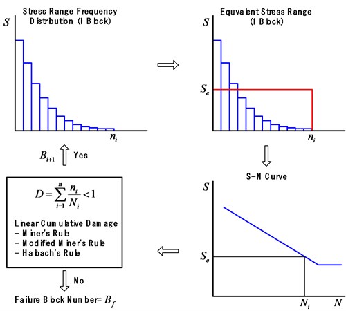
Fig. 1Procedure of fatigue reliability evaluation

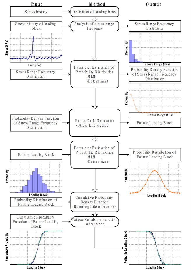
Stress range frequency analysis calculated the stress range frequency distribution from the stress history. The program developed for fatigue reliability evaluation technique has a Rainflow cycle count algorithm [14] to execute the stress range frequency analysis. A probabilistic method can be applied to the stress range frequency distribution, which is generated by the stress range frequency analysis [2, 9]. The Maximum Likelihood Method (MLM) ascertains the parameters of the probability distribution which expresses the stress range frequency distribution. The parameters for the Gumbel probability distribution, Lognormal, Exponential, and Weibull are estimated [17]. Fig. 1 shows the procedure for the fatigue reliability evaluation.

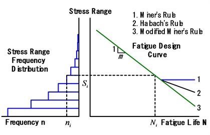
Generally, an S-N curve has been used for the fatigue design of steel structures [19] and has also been used together with the Miner’s Rule if it is required for fatigue reliability evaluation. The Miner’s Rule used to predict the fatigue life is defined as Eq. (1) [5, 14]:

1

D = \sum D_{i} = \sum \frac{n_{i}}{N_{i}} = 1, then f ailure state,

where $D$ is the summation of the damage index, $D_{i}$ is the fatigue damage index, $n_{i}$ is the frequency for the arbitrary stress range, and $N_{i}$ is the fatigue life. However, since the Miner’s Rule may be influenced less by the stress condition than by the fatigue threshold when the degree of fatigue damage becomes high, the Modified Miner’s Rule and the Haibach’s Rule as shown in Fig. 2 have been used to consider this type of effect.

Before defining the fatigue reliability, we need to consider that if $X$ is a failure loading block in a probability theory and $x$ is a loading block, the cumulative probability distribution of a failure loading block can be expressed by Eq. (2):

2

F_{X} (x) = P [X \leq x],

here $x$ refers to the loading block needed for failure. The fatigue reliability function $R_{X} (x)$ can be defined as Eq. (3):

3

R_{X} (x) = 1 - F_{X} (x) = 1 - P [X \leq x] .

Fig. 2Relationship between Stress Range and Fatigue Life by Linear Cumulative Damage

If the accumulative probability density function of destruction on the load block is given as the Weibull probability distribution, Eq. (3) can be modified to Eq. (5):

4

F_{X} (x) = 1 - e x p (- {(x / θ)}^{β}),

5

R_{X} (x) = 1 - F_{X} (x) = e x p (- {(x / θ)}^{β}) .

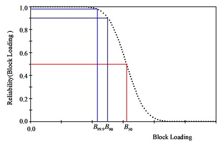
Using the fatigue reliability function, the failure loading block according to reliability (or a probability of failure in an opposite concept) can be calculated on the curve of a cumulative probability density function. Fig. 3 shows the curve of a cumulative probability density function of a failure loading block calculated by Monte Carlo Simulation (MCS). With the reliability of 99.9 %, the failure loading block is found to be $B_{99.9}$ , 90 % $B_{90}$ and 50 % $B_{50}$ in Fig. 3.

Fig. 3Fatigue reliability function

The failure loading block acquired for the equivalent stress range can be translated to the fatigue life in years by Eq. (6):

6

Y = \frac{B_{f}}{365 \times A D T T},

here $A D T T$ is the average truck traffic volume and $B_{f}$ is the failure loading block acquired by MCS.

In this paper, detail category and design fatigue strength were used in the design standard of highway bridges [3]. In the fatigue design instruction, this detail category has a slope of $m =$ 3 and a fatigue strength of stress cycle of 2×10⁶ at the design S-N curve. Because the design S-N curve of (average – 2 × standard deviation) was used in the fatigue life evaluation, the fatigue life was found to be short.

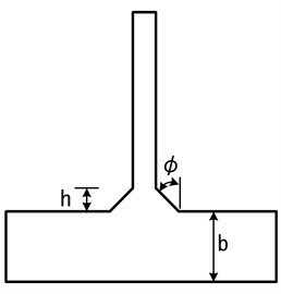
Fig. 4Connection category C

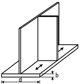
a)

b)

The analyzed member is the same as that in Fig. 4. According to the stress type and the detail category of the design standard of a highway bridge, when a member between a vertical stiffener and the bottom flange of a cross beam on a steel box girder bridge receives flexible stress of alternative or tensile stress, the allowable stress range is C degrees and the allowable stress range over 2 million cycles is 82.32 MPa.

The average daily traffic of the bridge of which the stress history was measured was 264 buses, 936 large trucks and 44,760 small cars. This bridge is a two span continuous girder bridge with a total of 4 lanes in both directions.

First, the stress history was measured on a welding member on the steel bridge located optimally for fatigue damage, as shown in Fig. 5.

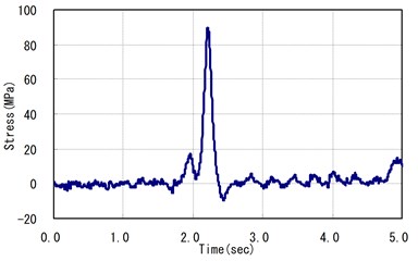
In particular, stress intensity occurs between the vertical stiffener and the bottom flange of the cross beam because the truck crossings create tensional stress in terms of deflection. Also, there may be fatigue damage possibility due to flaws in welding or to the effect of residual stress on the welding. The strain gauge on this part provided the strain history data. Strain history multiplied by Young’s modulus illustrates the stress history, as shown in Fig. 6.

Fig. 5Welding of a vertical stiffener and bottom flange of a cross beam

Fig. 6Stress history of a loading block

3. Fatigue reliability evaluation of a member

3.1. Stress range frequency analysis

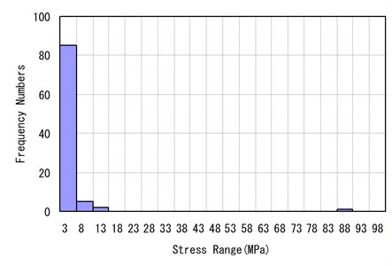
Stress history was modified starting from the maximum or minimum point, so that the half cycle of the stress range could not be counted. The frequency analysis of the stress range was performed by applying the Rainflow Cycle Count Algorithm [8, 10] and its results are shown on Fig. 7.

Fig. 7Stress range frequency distribution of a loading block

3.2. Probability distribution parameter estimation of stress range frequency distribution

Table 1 shows the Likelihood Function and the Maximum Likelihood Estimators for each probability distribution [13]. The stress range frequency analysis was performed for 400 loading blocks measured on the structural detail of a steel highway bridge. A probabilistic method was applied to the stress range frequency distribution. The objective of representing the frequency distribution of the stress range as a probability distribution is to enable Monte Carlo Simulation (MCS).

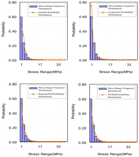
The probability distribution parameters were obtained by using the Maximum Likelihood Method (MLM) to find a particular probability distribution that adequately expresses the stress range frequency distribution. Each probability distribution is the Gumbel probability distribution, Lognormal, Exponential, and Weibull. Consequently, the Lognormal probability distribution sufficiently expressed the stress range frequency distribution of 400 loading blocks and then, the parameter $λ$ of Lognormal is 0.377, $ξ$ is 0.952, and the Determinant $r^{2}$ is 0.996. Table 2 shows the probability distribution parameters and Determinants. Fig. 9 shows the stress range frequency distribution of 400 loading blocks and each probability distribution curve.

Table 1Likelihood functions and parameters of probability distributions

Probability distribution	Likelihood function	Maximum likelihood estimator
Lognormal	$L (x_{1}, \dots, x_{n}; λ, ξ) = \prod_{i = 1}^{n} \frac{1}{\sqrt{2 π} ξ x_{i}} \exp [- \frac{1}{2} {(\frac{l n x_{i} - λ}{ξ})}^{2}]$	$\hat{λ} = \frac{\sum_{i = 1}^{n} l n x_{i}}{n}$ , ${\hat{ξ}}^{2} = \frac{1}{n} \sum_{i = 1}^{n} {(l n x_{i} - \hat{λ})}^{2}$
Exponential	$L (x_{1}, \dots, x_{n}; ω) = \prod_{i = 1}^{n} \frac{1}{ω} \exp (- \frac{x}{ω})$	$\hat{ω} = \frac{1}{n} \sum_{i = 1}^{n} x_{i}$
Weibull	$L (x_{1}, \dots, x_{n}; β, θ) = \prod_{i = 1}^{n} \frac{β}{θ} {(\frac{x}{θ})}^{β - 1} \exp [- {(\frac{x}{θ})}^{β}]$ .	$\frac{\sum_{i = 1}^{n} x_{i}^{β} l n x_{i}}{\sum_{i = 1}^{n} x_{i}^{β}} - \frac{1}{β} - \frac{1}{n} \sum_{i = 1}^{n} l n x_{i} = 0,$ $θ = \frac{\sum_{i = 1}^{n} x_{i}^{β}}{n}$
Gumbel	$L (x_{1}, \dots, x_{n}; α, φ) = \frac{1}{φ^{n}} ∙ \prod_{i = 1}^{n} \exp [- \exp (- \frac{x - α}{φ})] \exp (- \frac{x - α}{φ})$	$α = - φ \ln (\frac{1}{n} \sum_{i = 1}^{n} \exp (- \frac{x_{i}}{φ}))$ $φ - n^{- 1} \sum_{i = 1}^{n} x_{i} + \frac{\sum_{i = 1}^{n} (x_{i} \exp (\frac{- x_{i}}{φ}))}{\sum_{i = 1}^{n} \exp (\frac{- x_{i}}{φ})} = 0$

Table 2Determinants and parameters of each probability distribution for 400 loading blocks

Probability distribution	Gumbel		Lognormal		Exponential	Weibull
Parameters	$α$	$ψ$	$λ$	$ξ$	$ω$	$β$	$θ$
Parameters	1.370	1.308	0.377	0.952	0.439	1.064	2.475
Determinant ( $r^{2}$ )	0.834		0.996		0.993	0.976

3.3. Random number generation method

When using MCS, a procedure is needed to generate random numbers suitable for a distribution pattern of each random variable. After extracting a uniform random number between 0 and 1, this random number is translated properly to comply with a particular probability distribution. Here, the probability variable which complies with the probability distribution can be generated by producing a uniform random number and is translated into the variable of an appropriate probability distribution [6, 7, 12]. The standard normal distribution is universally used in statistical probability as well as in structure reliability theory, but because the probability distribution function is defined as an integral type, a general inverse transformation method cannot generate the random number of the standard normal distribution. Since the Lognormal Distribution is also given with the integral pattern of probability distribution function, the reciprocal transformation method is not available. Therefore, a random number for two distribution functions must be generated by a new method.

For the method where a uniform random number is generated, the Box Muller defined the uniform distribution random numbers, $U_{1}$ and $U_{2}$ , and showed that variables $Z_{1}$ and $Z_{2}$ are a pair of probability variables of each independent standard normal distribution [6]:

7

Z_{1} = \sqrt{- 2 l n (U_{1})} c o s (2 π U_{2}) or Z_{2} = \sqrt{- 2 l n (U_{1})} s i n (2 π U_{2}),

here $Z_{1}$ and $Z_{2}$ are random variables of the standard normal ( $μ =$ 0.0, $σ =$ 1.0). Therefore, Eq. (8) as follows can generate the random variable of nonstandard ( $μ = μ_{n s}$ , $σ = σ_{n s}$ ):

8

Z_{i} = σ_{n s} X_{i} + μ_{n s} .

In a different method, the pair of $V_{1} = 2 U_{1}$ – 1 and $V_{2} = 2 U_{2}$ – 1 represent the coordinates of a point which is assumed randomly in a square of points (1, 1), (1, –1), (–1, 1), (–1, –1). When $R = V_{1}^{2} + V_{2}^{2}$ is determined and is $R \leq 1$ , Eq. (9) can be used to calculate $Z_{1}$ and $Z_{2}$ :

9

Z_{1} = V_{1} {[- 2 \frac{l o g R}{R}]}^{\frac{1}{2}} or Z_{2} = V_{2} {[- 2 \frac{l o g R}{R}]}^{\frac{1}{2}},

where $Z_{1}$ and $Z_{2}$ are independent of N(0, 1). The probability variable of the lognormal probability distribution can be gained by using the above-mentioned uniform random number:

10

F_{X} (x) = \frac{1}{\sqrt{2 π} σ_{l n X}} \exp [- \frac{1}{2} {(\frac{l n x - μ_{l n X}}{σ_{l n X}})}^{2}] .

Fig. 8Stress range frequency distribution & each probability distribution for 400 loading blocks

Similarly, by following Eq. (11), which has a mean $μ$ and standard deviation $σ^{2}$ , the probability variable $X$ of the Lognormal probability distribution can be obtained:

11

X = e x p (λ + ξ \times Z),

12

ξ^{2} = l n [1 + {(\frac{σ}{μ})}^{2}], λ = l n μ - \frac{1}{2} ξ^{2} .

3.4. Probability distribution of failure loading blocks by MCS

The Lognormal probability distribution sufficiently expressed the stress range frequency distribution of 400 loading blocks, which were measured in the field. With the parameters of the stress range frequency distribution, MCS generated the probability variable of lognormal probability distribution and this numerical analysis acquired the degree of damage per loading block.

As shown in Fig. 9, after MCS generated the probability variable (stress range) of $n_{i}$ units for a loading block, it obtained the equivalent stress range. In particular, the Miner’s Rule of damage assessment method was used to calculate the equivalent stress range of the stress range over the fatigue limit. Subsequently, in the S-N curve, $D$ is calculated by $N_{i}$ and $n_{i}$ , which corresponds to the equivalent stress range ( $S_{e}$ ). MCS gains the failure loading blocks until $D$ is 1.0 by repetition:

13

S_{e} = \sqrt[m]{\frac{\sum S_{i}^{m} \cdot n_{i}}{\sum n_{i}}} .

Fig. 9Simulation procedure

Finally, because the variable that must be found is the failure loading block, when the damage index per loading block is 1.0, a structural member is considered to be broken and MCS finds the failure loading block. For these repeated works, the relation between Average Daily Truck Traffic ( $A D T T$ = 936) and the number of simulations (800, 1000, 2000, 5000, 10000, 20000 times) has been considered. The program of MCS was developed with Visual Basic 6.0.

After the probability distribution for failure loading blocks was estimated, lognormal probability distribution was adequately explained. Table 3 shows the lognormal probability distribution parameters according to ADTT and simulations. The probability distribution parameters of failure loading blocks were calculated by using MLM. Also, the Determinant evaluated the fitness degree of the probability distribution of the failure loading blocks.

Fig. 10 shows the Lognormal probability distribution curves and the probability distribution of failure loading blocks according to run = 1000 and $A D T T$ = 936. Fig. 11 shows the Lognormal cumulative probability distributions of failure loading blocks according to $A D T T$ = 936 and simulations. When run = 1000, a loading block with 0.5 (50 %) of the cumulative probability density is 2.1266×10⁷ by the Miner’s Rule, 1.7412×10⁷ by the Modified Miner’s Rule, and 1.9860×10⁷ by the Haibach’s Rule.

Table 3Lognormal probability distribution parameters according to simulations (Miner’s rule)

Simulations	Parameters of Lognormal probability distribution
Simulations	$λ$	$ξ$	$r^{2}$
800	16.888237	0.215602	0.952
1000	16.872628	0.217074	0.888
2000	16.881490	0.220668	0.939
5000	16.883257	0.217367	0.935
10000	16.880216	0.214844	0.962
20000	16.881594	0.220547	0.954

3.5. Calculations of member fatigue reliability

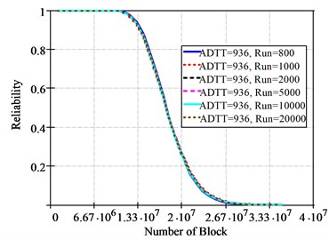
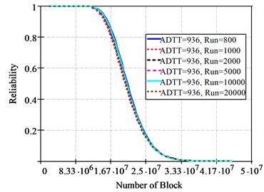
Fig. 12 shows the fatigue reliability curves of the Lognormal cumulative probability density according to run = 800, 1000, 2000, 5000, 10000, 20000 when $A D T T$ = 936. When run = 1000, the loading block with 0.9 (90 %) fatigue reliability is 1.6101×10⁷ by the Miner’s Rule, 1.3420×10⁷ by the Modified Miner’s Rule, and 1.5075×10⁷ by the Haibach’s Rule. Similarly to the failure cumulative probability density curves, the fatigue reliability curves are similar regardless of simulations.

3.6. Remaining life calculation of fatigue member

A fatigue damage index of 1.0 implies the failure of an objective member. In this study, after measuring the strain history produced by trucks of over 8-ton for 400 loading blocks, the stress range frequency distribution was obtained. Because the ADTT corresponds to 24 hours (a day), the traffic volume of the measurement day was representative (average) and afterward, this traffic situation was assumed to be continuous. Fatigue life is obtained by dividing the failure loading block into ADTT in the previous steps.

Data provided in Table 4 according to a fatigue reliability of 50 %, 90 %, and 99 % and run = 1000, $A D T T$ = 936, and fatigue life were obtained with the Miner’s Rule, Modified Miner’s Rule, and Haibach’s Rule of the damage assessment method. As expected, the fatigue life of the Modified Miner Rule was the smallest. The fatigue life of the Miner’s Rule assessment was larger than any other method because it ignored the stress range under the fatigue limit. In the Haibach’s Rule, fatigue damage is considered by prolonging the slope $m$ = 3 of the S-N curve for the stress range under the fatigue limit and the life of the Modified Miner’s Rule is smaller than that of Haibach’s Rule when slope $m$ = 5.

Table 4Fatigue life according to fatigue life estimation method (Run = 1000, ADTT = 936)

Damage assessment	Reliability (%)	Miner’s rule	Modified Miner’s rule	Haibach’s rule
Fatigue life (years)	50	62.24	50.96	58.13
	90	47.12	39.28	44.12
	99.9	31.90	24.29	29.85

3.7. Fitness of probability distribution and effect on simulations

Stress range is the major factor that dominates fatigue life. Because a particular probability distribution can express the stress range frequency distribution, Lognormal probability distribution sufficiently expressed the stress range frequency distribution of 400 loading blocks. Here, the fitness degree between the stress range frequency distribution and the theory probability distribution was judged by the Determinant ( $r^{2}$ ). In the case of 400 loading blocks, the Determinant of the Gumbel probability distribution was $r^{2}$ = 0.834, Lognormal 0.996, Exponential 0.993, and Weibull 0.976.

Fig. 10Failure probability distribution of ADTT = 936 and Run = 1000

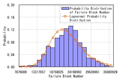
a) Miner’s rule

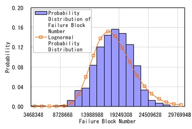
b) Modified Miner’s rule

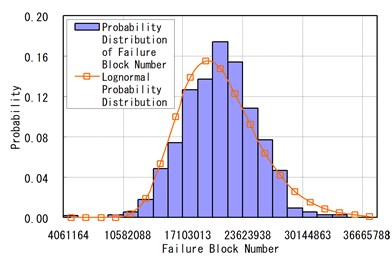
c) Haibach’s rule

Fig. 11Cumulative probability density of failure loading blocks according to simulations

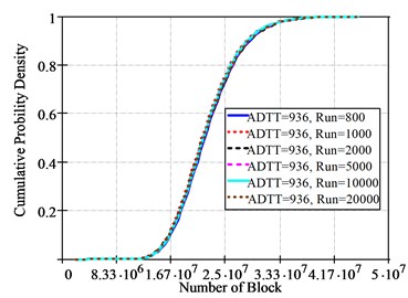
a) Miner’s rule

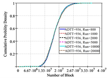
b) Modified Miner’s rule

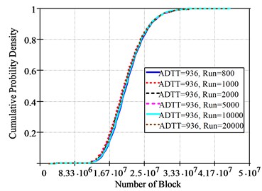
c) Haibach’s rule

Fig. 12Fatigue reliability according to simulations

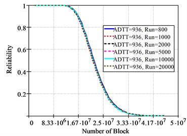
a) Miner’s rule

b) Modified Miner’s rule

c) Haibach’s rule

Fig. 13Relations among parameters, determinants and simulations

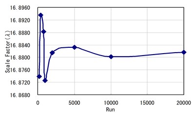
a) Relations between scale factor ( $λ$ ) and simulations

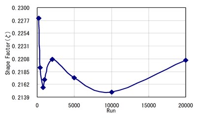
b) Relations between shape factor ( $ζ$ ) and simulations

c) Relation between determinant ( $r^{2}$ ) and simulations

Fig. 13 shows the influence of the Scale Factor ( $λ$ ), the Shape Factor ( $ζ$ ) of Lognormal probability distribution and the Determinant ( $r^{2}$ ) according to simulations. For the shape factors ( $ζ$ ) of a Lognormal probability distribution from Fig. 13(b), we can see that the $ζ$ value does not converge to a certain value according to the number of simulations. However, in Figs. 13(a) and 13(c), the Determinant and Scale Factor converge to a value as the number of simulations increases. Namely, the Determinant converged to a value after 2000 simulations.

4. Conclusions

In this study, the stress history was measured at the welding of the bottom flange and the vertical stiffener of a cross beam of a steel box girder bridge. A loading block was then defined and the probability method was applied to the stress range frequency distribution of the stress history. The fatigue reliability analysis model, which can compute the remaining life, the probability of fatigue failure and the reliability of the failure loading block gained by Monte Carlo Simulation, was brought forward. The fatigue reliability model assessed the structural detail, and conclusions are as follows.

1) Because the stress range frequency distribution of the loading blocks is a major factor of the dominating fatigue life, the probability distribution parameters of the stress range frequency distribution of 400 loading blocks were estimated by MLM. Consequently, Lognormal probability distribution was adopted as the probability distribution of the stress range frequency distribution and failure loading blocks. The Determinant, which was the criterion for judging the fitness degree, was larger than that of any other probability distribution.

2) From the parameters of Lognormal Distribution of Probability, Shape Factor ( $ζ$ ) does not represent any direct correlation to the number of simulations repeated. However, it appears that Scale Factor ( $λ$ ) and coefficient of determination ( $r^{2}$ ) are to be converted to a certain value when the numbers of simulations increase more than 2,000 times.

3) Monte Carlo Simulation, which can calculate the failure loading block with a probability distribution parameter of stress range frequency distribution, was appropriate for estimating the probability of failure of the fatigue member under a loading block and was the method chosen to easily carry out fatigue analysis.

References

Ariduru S. Fatigue Life Calculation by Rainflow Cycle Counting Method. Ph. D. Dissertation, The Graduate School of Natural and Applied Sciences of Middle East Technical University, 2004.

Search CrossRef
Barsom J. M., Rolfe S. T. Fracture and Fatigue Control in Structures. Applications of Fracture Mechanics. Prentice-Hall Inc., Englewood Cliffs, N. J., 1999.

Search CrossRef
Ellyin F. Fatigue Damage. Crack Growth and Life Prediction. Chapman & Hall, 2001.

Search CrossRef
Fricke W., Kahl A. Comparison of different structural stress approaches for fatigue assessment of welded ship structures. Marine Structures, Vol. 18, 2005, p. 473-488.

Search CrossRef
Fuchs H. O., Stephen R. I. Metal Fatigue in Engineering. John Wiley & Sons, 2000.

Search CrossRef
Gentle J. E. Random Number Generation and Monte Carlo Methods. Second Edition, Statics and Computing, Springer, 2004.

Search CrossRef
Haldar A., Mahadevan S. Reliability Assessment Using Stochastic Finite Element Analysis. John Wiley & Sons, Inc., 2000.

Search CrossRef
Korea Ministry of Construction & Transportation. Korea Design Standard of Highway Bridge. Korea Road & Transportation Association, 2005.

Search CrossRef
Laber S. The influence of surface layer on the surface fatigue strength of cast iron EN-GJSF. Journal of Vibroengineering, Vol. 13, Issue 3, 2011, p. 461-470.

Search CrossRef
Limbrunner J. F., Vogel R. M., Linfield C. B. Estimation of harmonic mean of a lognormal variable. J. Hydrologic Engrg., Vol. 5, Issue 1, 2000, p. 59-66.

Search CrossRef
Lin T. K., Wang Y. P., Huang M. C., Tsai C. A. Bridge scour evaluation based on ambient vibration. Journal of Vibroengineering, Vol. 14, Issue 3, 2012, p. 1113-1122.

Search CrossRef
Lukic M., Cremona C. Probabilistic assessment of welded joints versus fatigue and fracture. Journal of Structural Engineering, Vol. 127, No. 2, 2001, p. 211-212.

Search CrossRef
Mohammad A. A. Methods for estimating the parameters of the Weibull distribution. Science and Technology, 2000, p. 1-11.

Search CrossRef
Pourzeynali S., Datta T. K. Reliability analysis of suspension bridges against fatigue failure from the gusting of wind. J. Bridge Engrg., Vol. 10, Issue 3, 2005, p. 262-271.

Search CrossRef
Shimizu S. et al. New data analysis of probabilistic stress-life (P-S-N) curve and its application for structural materials. International Journal of Fatigue, Vol. 32, Issue 3, 2010, p. 565-575.

Search CrossRef
Sutherland H. J., Mandell J. F. The effect of mean stress on damage predictions for spectral loading of fiberglass composite coupons. EWEA, Special Topic Conference 2004, The Science of Making Torque from the Wind, Delft, April 19-21, 2004, p. 546-555.

Search CrossRef
Weibull W. Fitting of curves to observations. Fatigue Testing and Analysis of Results, New York: Pergamon Press, 1961, p. 201-203.

Search CrossRef
Yang Y. S., Seo Y. S., Lee J. O. Structure Reliability Engineering. Seoul National University Publication, 1999.

Search CrossRef
Zhou Y. E. Assessment of bridge remaining fatigue life through field strain measurement. J. Bridge Engrg., Vol. 11, Issue 6, 2006, p. 737-744.

Search CrossRef

About this article

Received

06 December 2012

Accepted

28 February 2013

Published

31 March 2013

Keywords

steel welding member

fatigue reliability

stress range frequency distribution

Acknowledgements

This research was supported by Chonnam National University as a University Grant in 2012-2013.

This is an open access article distributed under the Creative Commons Attribution License, which permits unrestricted use, distribution, and reproduction in any medium, provided the original work is properly cited.