Abstract
A real-time diagnosis of hydraulic pumps is very crucial for the reliable operation of hydraulic systems. The main purpose of this study is to propose a fault diagnosis approach for hydraulic systems based on the empirical mode decomposition (EMD), autoregressive (AR) model, singular value decomposition (SVD), and Mahalanobis–Taguchi system (MTS). The AR model effectively extracts the fault feature of vibration signals. However, it can only be applied to stationary signals; the fault vibration signals of hydraulic pumps are non-stationary. To address this problem, the EMD method is used as a pretreatment step to decompose the non-stationary vibration signals of hydraulic pumps. First, the vibration signals of hydraulic pumps are decomposed into a finite number of stationary intrinsic mode functions (IMF). The AR model of each IMF component is established. The AR parameters and the remnant’s variance are regarded as the initial feature vector matrices. Third, the singular values are obtained by applying the SVD to the initial feature vector matrices. Finally, these values serve as the fault feature vectors to be entered to the MTS, thereby classifying the fault pattern of the hydraulic pumps. The Taguchi methods are employed to reduce the redundant features and extract the principal components. Experimental analysis results indicate that this method can effectively accomplish the fault diagnosis of hydraulic pumps.
1. Introduction
A hydraulic pump is the heart of a hydraulic system. It reflects whether the operation of the entire system is normal or not. Therefore, hydraulic pumps should be able to process condition monitoring and fault diagnosis. Hydraulic pumps under an abnormal state are normally accompanied with vibration changes. Most mechanical faults are reflected by vibration. Thus, vibration diagnosis is important in this field and is also the foremost topic of interest for local and foreign researchers [1, 2]. In the fault diagnosis of hydraulic pumps, fault signals passed through the pump source outlet are often drowned by interference signals because of complex fault mechanisms and strong buzz during the signal extraction process. The effective fault characteristics are difficult to extract using conventional signal processing methods.
The hydraulic pump fault diagnosis process basically consists of three steps: (1) collection of the hydraulic pump vibration signals; (2) extraction of the fault features; and (3) pattern recognition and fault diagnosis. Steps 2 and 3 are the key steps in the fault diagnosis of hydraulic pumps. Considering that the fault vibration signals of hydraulic pumps are non-stationary, determining how to obtain feature vectors from these signals for fault diagnosis is important. Traditional diagnosis techniques obtain these vectors from the waveforms of the fault vibration signals in the time or frequency domain, and then construct the criterion functions to determine the condition of hydraulic pumps. However, considering that the non-linear factors have distinct effects on the vibration signals because of the complexity of the structure and working condition of hydraulic pumps, obtaining an accurate evaluation of the fault condition of hydraulic pumps only through time or frequency domain analyses is difficult.
In the timing analysis field, the autoregressive (AR) model is the most basic and most widely used time-series model, but it is mainly used in stationary processes. The AR model is a time sequence analysis method with mature algorithms whose parameters comprise important information regarding the system condition. An accurate AR model can reflect the characteristics of a dynamic system. The autoregression parameters of the AR model are also very sensitive to the condition variation [3, 4]. The vibration signals of hydraulic pumps with faults have shock characteristics. The AR model can simulate transients, and the frequency response function of these pumps can be calculated from the auto-regression parameters of the AR model. Therefore, these parameters can be effectively used to analyze the condition variation of dynamic systems. The most apparent advantage of the AR model is that faults can be identified by the AR model parameters after the AR model of the vibration signals is established without constructing mathematical models and studying the fault mechanisms. The AR model has also been successfully applied to fault diagnoses in many cases. When the AR model is applied to non-stationary signals, estimating the autoregression parameters by the least squares method or the Yule–Walker equation method is difficult; thus, the analysis results are inaccurate if the AR model is directly applied to non-stationary hydraulic pump vibration signals.
Signals generated by hydraulic pump failures traditionally often contain a large number of non-stationary components. The global frequency domain information can be obtained by performing a Fourier transform on the signals containing non-stationary components, but the fault information is difficult to be effectively extracted from a spectrum overwhelmed with noise. The local information of non-stationary signals can be extracted by wavelet transform. However, the high frequency information is lost because of the inability to decompose the high-frequency part; thus, the fault characteristics of high frequencies is difficult to be extracted. The wavelet packet transform compensates for the inability of the wavelet transform to decompose high frequencies. The wavelet packet transform can perform a complete multi-level decomposition in the full-band signal, coupled with good time-frequency characteristics. However, for some mechanical systems, this approach cannot obtain a vibration signal feature extraction with a high signal-to-noise ratio (SNR).
To get rid of the disadvantages of the feature extraction methods above, a self-adaptive method, namely, empirical mode decomposition (EMD), for nonlinear and non-stationary signals was proposed by Huang [5, 6]. In the present study, an effective method based on the EMD and AR model is presented to extract feature vectors. EMD is based on the local signal characteristics and could decompose complicated signals into a number of intrinsic mode functions (IMFs). The number of decomposed IMFs is usually finite, and the IMF components generated by EMD can reflect the actual information of the original signal. More importantly, the generated IMF components are stationary; thus, the AR model of each IMF component can be established. The initial feature vectors of the fault vibration signals of hydraulic pumps are extracted with the combination of EMD and the AR model. The feature vectors are composed of the autoregression parameters and remnant’s variance of the AR model. The feature vector matrices are decomposed to obtain the singular value by singular value decomposition (SVD).
The Mahalanobis–Taguchi system (MTS) is a multivariate pattern recognition tool that provides the basis to combine all the pertinent information about a system into a single metric using the Mahalanobis distance (MD). It also presents a systematic way of determining the key features required for analysis based on the Taguchi methods. MTS is widely used in various diagnostic applications that deal with data classification. In MTS, the MD is used to determine the degree of abnormality, thereby identifying the working condition and fault patterns of hydraulic pumps. The Taguchi methods use orthogonal arrays (OAs) and SNRs. These methods are also used to reduce the redundant features and extract the principal components. The MD, introduced by P. C. Mahalanobis in 1936 [7], is a multivariate generalized measure used to determine the distance of a data point to the mean of a group. The MD is measured in terms of the standard deviations from the mean of the samples and provides a statistical measure of how well the unknown data set matches with the ideal one. The advantage of the MD is that it is sensitive to the intervariable changes in the reference data. Therefore, it has traditionally been used to classify observations into different groups for diagnoses [8].
The benefits of MTS as a pattern recognition and data classification tool are summarized as follows.
• It is a robust methodology insensitive to variations in multidimensional systems.
• It can handle many different types of data sets and effectively consolidates these data into a useful metric.
• Implementation of MTS requires limited knowledge of statistics.
• It typically relies on simple arithmetic, contextual knowledge, and intuition.
• Its success has been demonstrated in various practical applications.
2. Methodologies for hydraulic pump fault diagnosis based on EMD-AR and MTS
2.1. EMD method
Huang et al. [5] developed EMD in 1998. The EMD method is developed based on the simple assumption that any signal consists of different simple intrinsic modes of oscillations. Each linear or non-linear mode will have the same number of extrema and zero-crossings. Only one extremum exists between successive zero-crossings. Each mode should be independent of the others. In this way, each signal could be decomposed into a number of IMFs, each of which must satisfy the following definitions [9]: (1) In the whole data set, the number of extrema and the number of zero-crossings must either be equal or differ by at most one; (2) At any point, the mean value of the envelope defined by the local maxima and the envelope defined by the local minima is zero.
An IMF represents a simple oscillatory mode compared with the simple harmonic function. With the definition, any signal can be decomposed as follows:
Step 1: Identify all the local extrema, and then connect all the local maxima by a cubic spline line to give the upper envelope.
Step 2: Repeat this procedure for the local minima to produce the lower envelope. Between them, the upper and lower envelopes should cover all the data.
Step 3: The mean of the upper and lower envelope values is designated as ; the difference between the signal and is the first component :
Ideally, if is an IMF, then is the first component of .
An equivalent set of two first-order non-autonomous equations is as follows:
Step 4: If is not an IMF, is treated as the original signal and steps 1, 2 and 3 are repeated; then:
After repeated sifting, i.e., up to times, becomes an IMF, that is:
Then, it is designated as:
The first IMF component from the original data should contain the finest scale or the shortest period component of the signal.
Step 5: Separating from , we get:
is treated as the original data, and the above processes are repeated; therefore, the second IMF component of can be obtained. Repeating the process described above times, -IMFs of signal can be obtained. Then:
The decomposition process can be stopped when becomes a monotonic function from which no more IMFs can be extracted.
Using this procedure, any signal can be decomposed. We finally obtain:
Thus, the signal is decomposed into -empirical modes and a residue , which is the mean trend of . Each IMF contains lower-frequency oscillations than the prior-extracted one, while represents the central tendency of signal .
EMD has been shown to be a fast, effective, self-adaptive method for nonlinear and non-stationary time series analysis, but there is still a drawback worth noting: the end effect, whereby distortion appears at the end of the signal in the decomposition process. In this paper, we employ the mirror periodic extending method (MPM) to solve this problem.
2.2. MTS
The MTS starts by collecting data on normal observations. The MD is calculated using certain characteristics to determine whether the MD has the ability to differentiate a normal group from an abnormal group. If the MD cannot identify the normal group using those particular characteristics, then a new combination of characteristics are needed to be examined. When the correct set of characteristics is determined, the Taguchi methods are employed to evaluate the effect of each characteristic. If possible, dimensionality is reduced by eliminating those characteristics that do not add value to the analysis. The MTS consists of the following three stages [8, 10].
2.2.1. Stage 1: Construction of the Mahalanobis Space (MS)
Step 1: Calculate the mean for each characteristic in the normal dataset as:
Step 2: Calculate the standard deviation , for each characteristic (1, 2, 3, …):
Step 3: Normalize each characteristic. Form the normalized data matrix , and take its transpose , where:
Step 4: Verify that the mean of the normalized data is zero:
Step 5: Verify that the standard deviation of the normalized data is one:
Step 6: Construct the correlation matrix , for the normalized data. Calculate the matrix elements , as follows:
Step 7: Calculate the inverse of the correlation matrix .
Step 8: Calculate MD as:
where is the th characteristic in the th observation, is the number of observations, is the standard deviation of the th characteristic, is the normalized value of the th characteristic in the th observations, is the standard deviation of the normalized values, is the correlation matrix is the inverse of the correlation matrix, is the MD for the th observation, and is the number of characteristics [11].
2.2.2. Stage 2: Identification of the useful characteristics
The useful characteristics are determined using OAs and SNRs. An OA is a table that lists the set of characteristics. It allows the effects of the presence or absence of a characteristic to be tested. The size of the OA is determined by the number of characteristics and the levels that they can take. In the MTS, characteristics in the OA have two levels. Level-1 represents the presence of a characteristic, and Level-2 represents the absence of a characteristic. For the abnormal cases, the MD values are calculated using the combination of the characteristics determined by the OA. The larger-the-signal-the-better SNR is calculated as follows:
where is the SNR for the row of the OA, and n is the sample size of each abnormality under the consideration of the Taguchi analysis. By obtaining the average SNRs at Level-1 () and Level-2 of each characteristic, the Gain in SNR can be calculated as . If , it means this characteristic is useful; otherwise, it is useless or even harmful for diagnosis. Thus, characteristics with positive gain are selected for the detection of abnormalities and the rest are discarded.
2.2.3. Stage 3: Decision making
In the final stage, the application under investigation is monitored by collecting data using the MS. The MDs are calculated, and if MD >> 1, the application exhibits an abnormal behavior and appropriate corrective actions are needed to be taken. If MD ≤ 1, then the conditions are normal [11].
2.3. Diagnosis approach for hydraulic pump
First, the fault vibration signal of the hydraulic pump , is decomposed by EMD into IMFs, . Each component represents a different characteristic information. After the EMD method is applied to , the IMFs can completely combine the characteristics of Therefore, the characteristics of can be obtained by extracting the characteristics of [9].
Second, the following AR model, , is established for each IMF component as:
where represent the parameters of the model, AR indicates an AR model of order , denotes the remnant of the model and is a white-noise sequence whose mean value is zero and variance is . The parameters can reflect the inherent characteristics of a hydraulic pump vibrating system. The variance of the remnant is closely related with the output characteristics of the system. and can be chosen as the initial feature vectors .
The singular values of the feature vector matrix are calculated to extract the feature vectors. Based on matrix theory, the singular value of the matrix is the inherent characteristic of the matrix and has good stability, that is, when the matrix elements encounter small changes, the matrix singular value only slightly changes. Thus, the singular values of the feature vector matrix obtained by AR can be extracted as mechanical component characteristics. However, the SVD also has its disadvantages, that is, for a space reconstruction in the time series, embedding dimension and delay decisions have no specific theoretical basis. The initial feature vector matrix obtained by AR could avoid this problem. Accordingly, the initial feature vector , from IMF components constitutes the initial feature vector matrix , where . is decomposed by SVD to extract the singular value , thereby extracting the fault feature vectors. The criterion of condition identification is the MD. The proposed diagnosis method is illustrated in Fig. 1.
The fault diagnosis method for the hydraulic pump is as follows:
(1) Acquire vibration signal samples at a certain sampling frequency , under each of the following conditions: hydraulic pump is normal, with valve plate wear, and with slipper loosing. The signals are taken as the samples.
(2) Each signal is decomposed by EMD, and finite number of IMF components can be obtained.
(3) Normalize each IMF component to obtain a new component to eliminate the effect of the signal amplitude on the variance of the remnant :
Fig. 1Flow chart of the proposed method
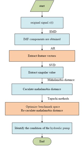
(4) Construct the AR model for the normalized component. Determine the order , of the model using the final prediction error (FPE) criterion and estimate the AR parameters and the remnant’s variance by the minimum squares method, where denotes the AR parameters of the IMF component. and can be determined. These values can be combined to construct the initial feature vector of the IMF component as follows:
where 1, 2, 3 denotes the normal condition, condition with valve plate wear, and condition with slipper loosing.
(5) Each sample in all conditions is decomposed by SVD to obtain singular values. Formally, the SVD of an real or complex matrix is a factorization of the form:
where is an real or complex unitary matrix, is an rectangular diagonal matrix with nonnegative real numbers on the diagonal, and (the onjugate transpose of ) is an real or complex unitary matrix. The diagonal entries of are known as the singular values of .
(6) Determine the MD between the testing data and the benchmark space composed of the normal training data as follows:
where is the inverse of the correlation matrix , is the MD for the observation, and is the number of characteristics.
(7) Establish the orthogonal table, optimize the benchmark space, reduce the redundant features, and extract the principal characteristics by Taguchi methods. The MD values for all of the datasets are re-calculated by using the optimized algorithm.
(8) Identify the fault condition of the hydraulic pump.
3. Case study
3.1. Experimental setup
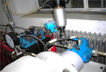
In this study, a test plunger pump rig, as shown in Fig. 2, was tested and analyzed to verify the presented fault diagnosis method. In the experiment, two commonly occurring faults in the plunger pump were set, namely, slipper loosing and valve plate wear. Under three conditions, including the two faulty conditions and the normal state, the vibration signal was acquired from the end face of the plunger pump with a stabilized motor speed of 528 r/min, and sampling rate of 1000 Hz. Twelve samples were acquired under the normal condition and four samples were obtained for each of the two fault states. Among these samples, the first eight normal samples were used to construct the benchmark space, and the remaining samples were used for testing.
Fig. 2Experimental test plunger pump rig
3.2. Feature extraction
The feature vectors were determined by the proposed method. The vectors were calculated using the first eight IMF components. Fig. 3 shows the acceleration vibration signal of the hydraulic pump with a normal signal. It is decomposed into eight IMFs by EMD. As shown in Fig. 4, each IMF component has a distinct time characteristic scale.
The system condition is mainly decided by the first several AR parameters and the remnant variance. The order of the model , was determined by FPE criterion. This order is different from the number of IMF components, wherein the maximum and minimum components are 26 and 9, respectively. In this case, the first seven AR parameters and were chosen. These values constitute the eight-dimension vector. The extracted feature vectors are listed in Table 1 (only the feature vectors of the first four IMF components from one sample in each condition are listed in Table 1 because of space limitations). denotes the feature vector of the IMF component under the condition, where denotes the normal condition, condition with valve plate wear, and condition with slipper loosing, and denotes the first eight IMF components. The feature vector matrixes were decomposed to obtain the singular value by SVD. The extracted singular values are listed in Tables 2 and 3. The extracted singular values for the model training (Table 2) are used to construct the benchmark space in calculating the MD, and the others (Table 3) are used for testing.
Fig. 3Acceleration vibration signal of the hydraulic pump with a normal signal
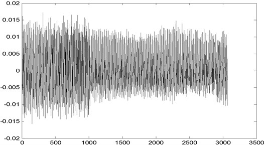
Fig. 4Decomposed results of the hydraulic pump vibration signal shown in Fig. 3 by EMD
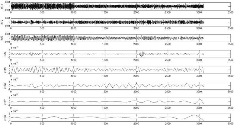
Table 1Feature vector components extracted by AR
Condition | Model feature vectors | Feature vectors components | |||||||
Normal | –0.414 | –0.1131 | –0.0102 | –0.1803 | 0.1412 | –0.0609 | –0.0462 | 0.1543 | |
1.6701 | –2.3772 | 2.2531 | –1.9891 | 1.4422 | –1.0649 | 0.615 | 0.0326 | ||
2.6695 | –3.3477 | 2.3751 | -1.2443 | 0.6057 | –0.245 | –0.1426 | 0.0451 | ||
3.6214 | –5.3801 | 4.3623 | –2.2972 | 0.8603 | –0.0995 | –0.1409 | 0.0210 | ||
Valve plate wear | 0.3393 | –0.2671 | 0.2528 | –0.1634 | 0.1845 | –0.2016 | 0.1769 | 0.2694 | |
2.5432 | –2.986 | 1.8495 | –0.8321 | 0.7009 | –0.7447 | 0.4229 | 0.0542 | ||
3.8075 | –6.0481 | 5.3307 | –3.0392 | 1.2048 | 0.1601 | –1.4367 | 0.0676 | ||
3.3826 | –3.6803 | 0.573 | –1.3447 | -0.3651 | –0.6244 | 0.5474 | 0.0310 | ||
Slipper loosing | –0.4318 | –0.0636 | 0.0609 | –0.1346 | 0.1154 | –0.1371 | –0.1563 | 0.3576 | |
2.0283 | –2.7278 | 2.9309 | –2.697 | 2.0974 | –1.6622 | 1.028 | 0.0754 | ||
2.9621 | –4.1079 | 3.5071 | –2.5696 | 2.0354 | –1.4728 | 0.6841 | 0.0678 | ||
3.9105 | –6.397 | 5.7949 | –3.3625 | 1.2503 | 0.2273 | –1.1323 | 0.0431 | ||
Table 2Extracted singular values for model training
Sample | Condition | 1 | 2 | 3 | 4 | 5 | 6 | 7 | 8 |
1 | Normal | 11.4321 | 5.8741 | 1.9654 | 1.0453 | 0.3001 | 0.3540 | 0.5671 | 1.1201 |
2 | 11.2650 | 6.0647 | 2.1096 | 1.0811 | 0.2655 | 0.4071 | 0.6304 | 1.3451 | |
3 | 11.4532 | 6.0421 | 1.9846 | 1.1546 | 0.3176 | 0.3679 | 0.6016 | 1.2306 | |
4 | 10.9546 | 6.0675 | 2.1326 | 1.1030 | 0.2709 | 0.4101 | 0.5977 | 1.3403 | |
5 | 11.0401 | 5.8154 | 2.0537 | 1.2574 | 0.3371 | 0.3791 | 0.5398 | 1.0756 | |
6 | 10.7416 | 5.8150 | 2.0529 | 1.0396 | 0.3259 | 0.4016 | 0.5343 | 1.2035 | |
7 | 11.5783 | 5.9074 | 1.8095 | 1.1277 | 0.3123 | 0.4044 | 0.5673 | 1.1431 | |
8 | 10.4506 | 6.0012 | 1.9901 | 1.2384 | 0.3451 | 0.3982 | 0.5512 | 1.3805 |
Table 3Extracted singular values for testing
Sample | Condition | 1 | 2 | 3 | 4 | 5 | 6 | 7 | 8 |
1 | Normal condition | 11.9631 | 6.0741 | 1.8647 | 1.1554 | 0.3204 | 0.3815 | 0.5250 | 1.3341 |
2 | 11.2403 | 6.1434 | 2.0743 | 1.2675 | 0.2447 | 0.4179 | 0.6089 | 1.5656 | |
3 | 10.9551 | 6.3268 | 1.9337 | 1.1396 | 0.3266 | 0.3445 | 0.6649 | 1.0105 | |
4 | 11.9760 | 6.0181 | 2.1326 | 1.2820 | 0.2984 | 0.4316 | 0.5960 | 1.2872 | |
1 | Valve plate wear | 11.2331 | 3.9450 | 3.0629 | 1.0377 | 0.6026 | 0.3201 | 0.0671 | 0.1305 |
2 | 11.2056 | 3.0837 | 3.2221 | 1.0879 | 0.6924 | 0.3748 | 0.0663 | 0.1346 | |
3 | 11.3034 | 2.9644 | 3.1108 | 0.9116 | 0.5886 | 0.2995 | 0.0552 | 0.1268 | |
4 | 11.9429 | 3.2617 | 3.1180 | 0.9225 | 0.7066 | 0.2959 | 0.0772 | 0.1363 | |
1 | Slipper loosing | 16.6911 | 3.6607 | 3.1738 | 1.5242 | 0.9463 | 0.4457 | 0.1703 | 0.0341 |
2 | 15.9531 | 3.3237 | 2.9694 | 1.6792 | 0.9242 | 0.4666 | 0.1503 | 0.0454 | |
3 | 15.2329 | 3.6717 | 2.3824 | 1.4922 | 1.1201 | 0.5919 | 0.2184 | 0.0465 | |
4 | 15.9614 | 4.2698 | 3.0456 | 1.6257 | 1.2857 | 0.5296 | 0.2710 | 0.0326 |
3.3. Pattern recognition
3.3.1. Fault diagnosis based on the MD
After obtaining the feature vectors using the proposed methods, the MD values of the testing samples for the three conditions can be obtained. The experimental results are listed in Table 4, wherein the MD between all the testing samples (Table 3) and the benchmark space composed of the trained normal samples (Table 2) are shown. Table 4 contains the mean, minimum, and maximum MDs for the three conditions. Separating the three conditions is easy by comparing the sizes of the MD values. These results verified that the MD method is very effective for fault detection and isolation.
Table 4Mean, minimum and maximum MD values
Normal condition | Valve plate wear | Slipper loosing | |
Mean | 2.9745 | 6.3752e+3 | 1.4668e+4 |
Min-max | 2.0645 – 4.2103 | 5.8055e+3 – 6.5876e+3 | 0.9707e+4 – 1.8737e+4 |
3.3.2. Algorithm optimization by Taguchi methods
First, the appropriate OA is selected, which is used for the two abnormal datasets to identify which characteristic is useless. Considering the different characteristics of each line measuring project, nine different benchmark spaces are formed. The larger-the-better SNR is calculated. Tables 5 and 6 show the results of the OA and SNR analysis for the valve plate wear and slipper loosing testing datasets. and in Tables 5 and 6 respectively denote the sum of the measurement feature project SNRs in Level-1 and Level-2.
From Tables 5 and 6, the energies of the 6th and 7th band should be excluded from the feature vector because they do not display a positive SNR for fault diagnosis. After the key features were identified, the MD values for all of the testing datasets were recalculated. The comparison between the initial and optimized MDs for each dataset is listed in Table 7. The optimized MDs are more stable and distinguishable than the initial MDs, thereby verifying that the Taguchi methods are very effective in reducing the redundant characteristics and extracting the principle components. Therefore, MTS can effectively conduct a fault diagnosis of hydraulic pumps.
Table 5Results of the OA and SNR analysis for the valve plate wear dataset
1 | 2 | 3 | 4 | 5 | 6 | 7 | 8 | SNR | |
1 | 1 | 1 | 1 | 1 | 1 | 1 | 1 | 1 | 29.37 |
2 | 1 | 1 | 1 | 1 | 1 | 2 | 2 | 2 | 50.38 |
3 | 1 | 1 | 2 | 2 | 2 | 1 | 1 | 1 | 28.82 |
4 | 1 | 2 | 1 | 2 | 2 | 1 | 2 | 2 | 14.68 |
5 | 1 | 2 | 2 | 1 | 2 | 2 | 1 | 2 | 16.18 |
6 | 1 | 2 | 2 | 2 | 1 | 2 | 2 | 1 | 24.08 |
7 | 2 | 1 | 2 | 2 | 1 | 1 | 2 | 2 | 25.43 |
8 | 2 | 1 | 2 | 1 | 2 | 2 | 2 | 1 | 26.81 |
9 | 2 | 1 | 1 | 2 | 2 | 2 | 1 | 2 | 21.87 |
27.25 | 30.45 | 29.08 | 30.69 | 32.32 | 24.58 | 24.06 | 27.27 | ||
24.70 | 18.31 | 24.26 | 22.98 | 21.67 | 27.86 | 28.28 | 25.71 | ||
2.55 | 12.13 | 4.81 | 7.71 | 10.64 | -3.29 | -4.22 | 1.56 | ||
Useful | Y | Y | Y | Y | Y | N | N | Y |
Table 6Results of the OA and SNR analysis for the slipper loosing dataset
1 | 2 | 3 | 4 | 5 | 6 | 7 | 8 | SNR | |
1 | 1 | 1 | 1 | 1 | 1 | 1 | 1 | 1 | 55.04 |
2 | 1 | 1 | 1 | 1 | 1 | 2 | 2 | 2 | 48.57 |
3 | 1 | 1 | 2 | 2 | 2 | 1 | 1 | 1 | 28.78 |
4 | 1 | 2 | 1 | 2 | 2 | 1 | 2 | 2 | 24.85 |
5 | 1 | 2 | 2 | 1 | 2 | 2 | 1 | 2 | 26.36 |
6 | 1 | 2 | 2 | 2 | 1 | 2 | 2 | 1 | 35.15 |
7 | 2 | 1 | 2 | 2 | 1 | 1 | 2 | 2 | 24.67 |
8 | 2 | 1 | 2 | 1 | 2 | 2 | 2 | 1 | 38.91 |
9 | 2 | 1 | 1 | 2 | 2 | 2 | 1 | 2 | 25.95 |
36.46 | 36.99 | 38.60 | 42.22 | 40.86 | 33.34 | 34.03 | 39.47 | ||
29.84 | 28.79 | 30.77 | 27.88 | 28.97 | 34.99 | 34.43 | 30.08 | ||
6.61 | 8.20 | 7.83 | 14.34 | 11.89 | -1.65 | -0.40 | 9.39 | ||
Useful | Y | Y | Y | Y | Y | N | N | Y |
Table 7Comparison between the initial and optimized MDs
Normal condition | ||
Initial | Optimized | |
Mean | 2.9745 | 0.8750 |
Min-max | 2.0645 – 4.2103 | 0.3958 – 1.0156 |
Valve plate wear | ||
Initial | Optimized | |
Mean | 6.3752e+3 | 5.1592e+2 |
Min-max | 5.8055e+3 – 6.5876e+3 | 3.1254e+2 – 5.9355e+2 |
Slipper loosing | ||
Initial | Optimized | |
Mean | 1.4668e+4 | 1.2638e+3 |
Min-max | 0.9707e+4 – 1.8737e+4 | 0.7084e+3 – 1.5321e+3 |
4. Conclusions
The characteristic information of the hydraulic pumps can be effectively isolated and highlighted by EMD-AR and SVD combined with MTS. The AR model simulates the characteristics and working condition of hydraulic pump systems. However, the AR model can only analyze stationary signals; thus, in this study, a pretreatment on the vibration signals is carried out by EMD before the AR model is established. The IMF components not only reflect the actual information contained in the signal, but are also stationary. The IMF components obtained by EMD highlights the different local characteristic information of the original signal, which is useful for fault feature extraction. Using the AR model combined with SVD not only accurately reflects the hydraulic pump operation state, but also significantly compresses the input dimension of the MTS. The Taguchi methods offer a systematic way to determine the principal features based on the MD, which is a more effective method for fault diagnosis.
References
-
S. P. Wang, Z. K. Yuan, G. Q. Yang Study on fault diagnosis of data fussion in hydraulic pump. China Mechanical Engineering, Vol. 16, Issue 4, 2005, p. 327-331.
-
W. L. Jiang, S. Q. Zhang, Y. Q. Wang Wavelet transform method for fault diagnosis of hydraulic pump. Chinese Journal of Mechanical Engineering, Vol. 37, Issue 6, 2001, p. 34-37.
-
H. Ding, Y. Wu, S. Z. Yang Fault diagnosis by time series analysis. Applied Time Series Analysis, World Scientific Publishing Co., Singapore, 1989.
-
Y. Wu, S. Z. Yang Application of several time series models in prediction. Applied Time Series Analysis, World Scientific Publishing Co., Singapore, 1989.
-
N. E. Huang, Z. Shen, S. R. Long A new view of nonlinear water waves: the Hilbert spectrum. Annual Review of Fluid Mechanics, Vol. 31, 1999, p. 417-457.
-
P. C. Mahalanobis On the generalized distance in statistics. Proceedings, National Institute of Science of India, Vol. 21, p. 49-55.
-
G. Taguchi, R. Jugulum The Mahalanobis–Taguchi strategy. A Pattern– Technology System, Wiley, New York, 2002.
-
N. E. Huang, Z. Shen, Steven R. Long The empirical mode decomposition and the Hilbert spectrum for nonlinear and non-stationary time series analysis. Proc. R. Soc. Lond., Vol. 454, Issue 1971, 1998, p. 903-995.
-
J. S. Cheng, D. J. Yu, Y. Yang A fault diagnosis approach for roller bearings based on EMD method and AR model. Mechanical Systems and Signal Processing, Vol. 20, Issue 2, 2006, p. 350-362.
-
G. Taguchi, S. Chowdury, Y. Wu The Mahalanobis Taguchi System. McGraw-Hill, New York, 2001.
-
S. Ahmet, S. Jagannathan Mahalanobis Taguchi system (MTS) as a prognostics tool for rolling element bearing failures. Journal of Manufacturing Science and Engineering, Vol. 132, Issue 5, 2010.
About this article
This study is supported by the National Natural Science Foundation of China (Grant Nos. 61074083, 50705005 and 51105019) and by the Technology Foundation Program of National Defense (Grant No. Z132010B004).
