Abstract
A strategy for the selection of optimal smoothing parameter for hybrid experimental-numerical photoelastic experiment is proposed in this paper. This is not a straightforward procedure for photoelastic analysis since conventional finite element techniques are based on the approximation of nodal displacements, not stresses. Although the displacements are continuous at inter-element boundaries, the calculated stresses are discontinuous due to the operation of differentiation.
1. Introduction
Hybrid numerical–experimental photoelastic analysis is an attractive methodology evaluating the quality of the structural design in terms of the stress distribution. But conventional finite element analysis techniques are based on the approximation of nodal displacements (not stresses) via the shape functions. Ramesh et al. [1] have noted that photoelastic fringes can be effectively used for the detection of FEM meshing problems. Several different strategies for the selection of the photoelastic smoothing parameter have been proposed (a short overview of these strategies is given in the next section). Nevertheless a subjective and interactive human assessment of the reconstructed field of photoelastic fringes is required for all these methodologies before the final decision regarding the acceptable smoothing is taken. Therefore there exists a need for an effective objective data driven strategy for the selection of optimal smoothing parameter and this paper gives a qualitative description of such a technique.
2. Preliminaries
A finite element norm [2] can be exploited for the adaptive selection of the smoothing parameter, which characterizes the error of reconstructed stress field. First, using the least squares method the nodal stress values can be identified in the global domain by minimizing the differences between the interpolated stress fields calculated on the basis of the values of nodal stresses and the theoretically calculated stress values based on the displacement field. Since the minimization is performed in the global domain and the interpolation is performed in the local domain of each element, the direct stiffness procedure can be applied for the described problem.
The common stress field calculation method is based on the global minimization of error calculated as the integral of the squared difference between the interpolated and factual stress fields:
here means FEM direct stiffness procedure; integrals are calculated in the domain of each finite element; is the shape function series of the finite element; is the column of the nodal values of the finite element stress components, and are the coordinates of the two-dimensional coordinate system.
The calculated nodal stress values, the finite element norms are calculated for each element as the average error of the field reconstruction, obtained by interpolating these nodal values. The first step of the calculation of nodal stress value creates a continuous stress field in the global domain. Nevertheless this field is purely suitable for visualization procedures, because the partial derivatives of the field are discontinuous on the inter-element boundaries, therefore during visualization the fringes become broken. The smoothing method proposed in [3] is based on the extension of the minimized error by a penalty for a rapid change of stress value in any analyzed direction:
here are smoothing parameters selected individually for each finite element, – the number of finite elements in the global structure. The choice of the smoothing parameter is performed interactively from the qualitative view of the digital photoelastic images. When the parameter is too small the images are of unacceptable quality because of the unphysical behavior of the stress fields as a result of their calculation from the displacement formulation. When the parameter is too big an over-smoothed image is obtained which may look acceptable but be far from the real photoelastic image. So the best value of the parameter might be considered when most of the image is of acceptable quality without the unphysical behavior produced by the approximation. The smoothing parameter can be interpreted as a small penalty parameter to prevent the growth of derivatives of each component of the stresses:
where is the smoothing parameter; – the global vector of nodal values of ; – the global vector of nodal values of ; – the global vector of nodal values of ; – the row of the shape functions of the finite element; and – the matrix of the derivatives of the shape functions:
It can be noted that when the parameter of smoothing is too small the reconstructed images are of unacceptable quality because of the non-physical behavior of the stress field as a result of its calculation from the displacement formulation. When the parameter is too big an oversmoothed image is obtained, which may look acceptable but is far from the real photoelastic image. The components of the stresses can be interpolated from their nodal values by using the shape functions of the finite element. Then the components of strains , , and are obtained using those values of stresses and the matrix of elastic constants:
Then the relative error norm for the -th finite element can be calculated as [4]:
For those parts of the image where the relative error norms of the finite elements are too large, the image is expected to be of insufficient quality and a finer meshing or smoothing of the image with a larger value of the smoothing parameter may be required. The selection of the smoothing parameter is then straightforward:
where function can be selected as a linear growing function, . The slope of the function depends on the meshing and particularly on the type of the finite element used.
3. The proposed technique
We will illustrate the proposed smoothing technique based on a simple one-dimensional example. Let us consider the following structure comprising 3 finite elements shown in Fig. 1.
Fig. 1The illustrative example comprising 3 quadratic finite elements
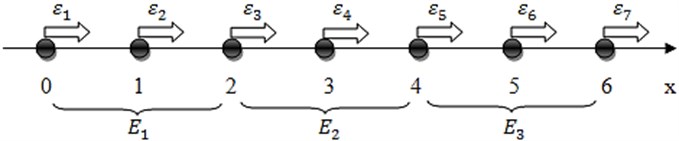
Nodal coordinates are set as follows: , . Then the shape functions for the -th element read:
where . The distribution of strain in the -th element is expressed as:
Thus, stresses in the domain of the -th element read:
where:
Let us denote the unknown nodal values of stresses as . Then:
and:
Nodal values of stresses are computed from the linear algebraic system (Eq. (3)). Then the smoothed field of stresses in the domain of the -th element reads:
Fig. 2Discontinuous theoretical stress field (the solid line) and the regularized stress field (the dashed line)
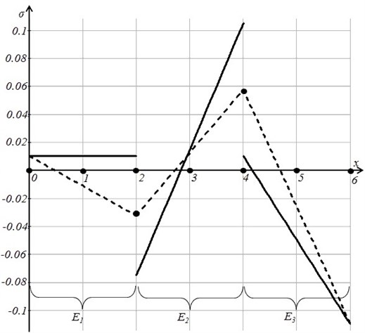
Let us assume that Then the graphical representation of the theoretical and regularized fields of stress is shown in Figure 2. Note that the regularized field of stress is constructed as the interpolation of nodal values of stresses, computed as the arithmetic average of the values of the theoretical field of stresses at corresponding nodes.
Now we minimize the residual computed as the difference between the nodal values of the regularized field (denoted as ) and the smoothed nodal values :
The smoothed fields of stresses at 0 and 0.032 are illustrated in Figure 3.
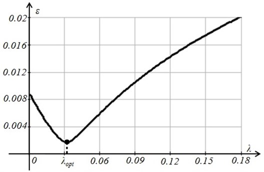
Finally it can be noted that 0.032 is the optimal value of the photoelastic smoothing – the variation of with respect to is shown in Figure 4.
Fig. 3The smoothed field of stresses at λ= 0 (the thin solid line) and at λ= 0.032 (the thick solid line) shown together with the regularized field (the dashed line)
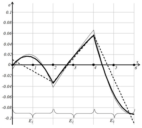
Fig. 4Minimation of the residual R with respect to the smoothing parameter λ
4. The application of the technique for a 2D structure
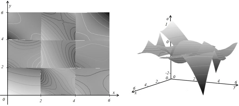
The proposed technique for the optimal selection of the smoothing parameter can be effectively implemented for a more complex FEM analysis. We will illustrate this technique using a 2D FEM structure comprising 9 Lagrange finite elements with quadratic interpolation. The theoretical field of stresses is continuous in the domain of every element, but discontinuous at inter-element boundaries (Figure 5).
Fig. 5The theoretical field of stresses is continuous in the domain of each finite element, but is discontinuous at inter-element boundaries
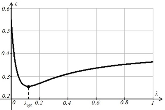
The variation of the residual (Eq. (12)) with respect to is shown in Figure 6; the optimal value of the smoothing coefficient is 0.124.
Fig. 6The minimal value of the residual R is reached at λopt= 0.124
Finally the smoothed fields of stresses at 0 and 0.124 are illustrated in the Figures 7a and 7b.
Fig. 7The smoothed fields of stresses at λ= 0 (part a) and λopt= 0.124 (part b)
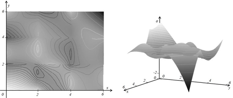
a)
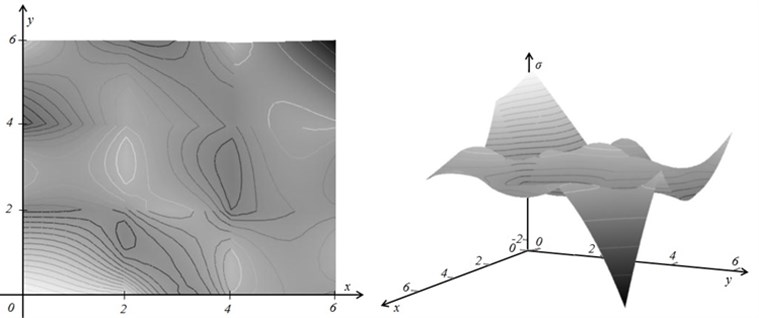
b)
5. Conclusions
The digital smoothing of photoelastic stresses produced by the finite element method is an important part of hybrid experimental-numerical methods for measurement of engineering structures. A number of different approaches for qualitative smoothing of the photoelastic fringes had been proposed during the last decade. Our approach belongs to the same group of problems, but the value of the smoothing parameter is selected not on the basis of the subjective visual interpretation of the smoothed image, but on the minimization of the residual assessing differences among nodal values of theoretical and regularized stresses. Such an approach fits well into the modular structure of finite element algorithms and can be effectively exploited in different photoelastic measurement scenarios.
References
-
Ramesh K., Pathak P. M. Role of photoelasticity in evolving discretization schemes for FE analysis. Journal of Experimental Techniques, Vol. 23, Issue 4, 1999, p. 36-38.
-
Bathe K. J. Finite Element Procedures in Engineering Analysis. Prentice-Hall, New Jersey, 1982.
-
Ragulskis M., Ragulskis L. Conjugate approximation with smoothing for hybrid photoelastic and FEM analysis. Communications in Numerical Methods in Engineering, Vol. 20, Issue 8, 2004, p. 647-653.
-
Ragulskis M., Ragulskis L. Plotting isoclinics for hybrid photoelasticity and finite element analysis. Experimental Mechanics, Vol. 44, Issue 3, 2004, p. 235-240.
About this article
