Abstract
Due to population growth in major cities, many issues and problems bother related governors. Due to noise pollution, diseases like psychiatric, hearing problems and sleep disorders increased dramatically. In conclusion, this issue has to be studied and controlled by authorities in order to increase health care of area. This paper is case study of sound wave emission of one of the most crowded highways in Tehran city. In result, in rush hours, when the volume of vehicles is in its most and their speed in low, noise pollution of the area increases. But when the road in clear and speed in high and volume is low, sound level reaches its lowest value. Average sound level of this highway is 97.23 (dB).
1. Introduction
These days, due to population growth in major cities, many issues and problems bother related governors. At first glance, it may not seem very important. But the consequences of its presence in the community can be very serious. Neurological and psychiatric diseases, hearing problems and sleep disorders are effects of noise pollution in the area [1]. There are many noise resources exist in environment and to reduce their effects in the area, there are several methods. Roads are one of the most effective noise emission resources in cities. For noise emission reduction, several methods are conducted by authorities and they were successful. One way, which is common in Tehran, is installing sound barriers in road sides. Special design of these barriers, give them ability to entrap sound waves in roadway and avoid them to emit in area [2]. In this method, production and installation of these barriers will cost time and money more than usual project. Another method which is well known around the globe and is used in many countries is using porous asphalt. Due to the high ratio of pores in this type of asphalt, the sound wave, which is produced by vehicles mainly as a result of rolling of tiers, is entrapped in the superstructure and its energy is consumed and consequently less noise is produced [3]. This project was for the first time launched in Spain and United States. It was later developed and the technical specifications, grading and quality of materials used in this asphalt were also spread [4]. The primary cost of application of this asphalt is lower than that of construction of sound barriers. However, the maintenance costs associated with this method are higher in the long run [3]. Different methods are employed in order to assess and select a suitable method for controlling noise pollution in a region. The common method of calculating noise pollution in the case of roads is the use of traffic parameters such as velocity and volume. Some studies examined the relationship between noise and the flow-velocity curve and presented models based on the results [5]. In some studies, the genetic algorithm and the artificial neural network model were used to design a model of noise diffusion model [6]. However, among all these models, models designed on the basis of average velocity and traffic volume are more common. The reason is that they are easy-to-use in traffic studies and provide satisfactory precision in the prediction of noise pollution of the region. The SMM1 model is one of such models [7]. This model was used for noise pollution modeling in different cities in the world, including Tehran [8]. In this research, it was tried to propose a noise modeling for the study area so as to examine and analyze the conditions of the region. In the following, the research problem is stated and the associated problems and issues are also discussed.
2. Problem statement
The primary objective of this research was to calculate the noise pollution in the vicinity of a highway located in Tehran. This objective was pursued by modeling noise pollution diffusion on the basis of traffic parameters. Numerous models are employed in different countries. These models are developed by considering factors influencing noise pollution in the countries. Hence, the applied model used for calculation of noise varies by country [7]. For example, in Vietnam, motorcycle is a major cause of diffusion of noise in cities [9]. In general, results of different studies suggest that the level of noise in the developing country is higher than in the developed countries. The reason is that the number of motorcycles crossing cities of low-income developing countries is high [10]. However, the model used in this research complies with the conditions governing Tehran City and thus its parameters also conform with the study area. Therefore, in this study it was first tried to obtain a model for calculation of noise pollution in the city of Tehran with regard to the unique traffic conditions of this city. Afterwards, a case study was carried out on a highway in this city and the equivalent level of noise in the surroundings was calculated. In order to assess the precision of the model, the study area was assessed using a sound meter and a comparison was drawn between the result of the model and the measured values.
3. Research method
3.1. Noise diffusion model
From the studies on the models designed by different countries, the SMM1 model was selected for the study area (Tehran). This model was developed in Germany for noise modeling. In this country, two models are used for modeling noise pollution. The first model, which was used in this research, is simpler because it involves fewer calculation parameters. The advantages of using this model include the high speed and satisfactory precision of noise calculation. The second model involves many parameters which add to the complexity and difficulty of the model. This model is highly precise but it is time-consuming and expensive [8]. Since the calculation precision provided with the first method was suitable for the purpose of this model and since it provides for high-speed calculations, this model was used to calculate noise pollution diffusion in the study area. In this model, vehicles are divided into three categories: light-weight, medium-weight (e.g. uniaxial trucks and buses), and heavy-weight (e.g. multi-axial trucks and trailers). The first, second and third categories are shown by , , and in the set of traffic parameters, respectively. Each of the mathematical equations provided in the following incorporates signs and symbols. These symbols and abbreviations are also explained for the ease of understanding. The output of calculations is a figure equal to the equivalent level of noise. It is expressed in terms of decibels and is shown by .
The equivalent noise level is obtained as follows [11]:
In the above relation, the only unknown variable, which is of concern in this research, is the equivalent level of sound, which is shown by . Other parameters on the other side of the equation include parameters that can be calculated on the basis of traffic criteria. In the following, each parameter as well as the relevant calculation method is explained. In this equation, denotes the calculated noise, which normally falls in three different periods. The average value of is known as the average total noise per day. Following the calculations, +5 dB and +10 dB are added to the results obtained for evening and night, respectively. This modification is aimed to enhance the convenience of people of the region. The value of is calculated through the following relation:
where, , and refer to the noise spread by light-weight, medium-weight and heavy-weight vehicles, respectively. Each of these values can be calculated separately through the following equations:
where, is the speed limit (80 km/h for light weight vehicles and 70 km/h for medium- and heavy-weight vehicles). In addition, , and also stand for the average speed values regardless of time for light-, medium-, and heavy-weight vehicles, respectively. Finally, the value of or noise can be easily obtained following the aforementioned three calculations through modifications aimed to ensure comfort and convenience of the surroundings. On the other hand, is also the correction factor for the type of asphalt, which is calculated according to the following Table 1.
Table 1Pavement correction in each classification
Pavement correction | Pavement classification | Noise level correction | ||
Porous | 0-60 km/h | 61-80 km/h | 81-130 km/h | |
–1 (dB) | –2 (dB) | –3 (dB) | ||
Fresh pavement (Asphalt or cement) | 0 (dB) | |||
Old pavement (Asphalt or cement) | 2 (dB) | |||
Corrugated cement | 2 (dB) | |||
Stone pavement | 3 (dB) | |||
The concern of the discussions included in this study and the result of observations suggest that this correction makes a difference when the asphalt is fresh or old. The difference is a result of the wider porous area in the case of fresh asphalt. Over time, as vehicles go over the superstructure, the concentration of the superstructure is increased and its porosity decreases. Consequently, the noise pollution in the environment escalates accordingly. However, in the early days of the life of the asphalt layer, the increasing trend of noise pollution is more than the ending days of the life of the asphalt layer. The reason is that at the beginning of operation of the superstructure and traffic of vehicles, the level of threshing and compaction is higher than the end of the life of layer.
is the correction resulting from the noise of braking or increased speed of the vehicle. This is also called the correction factor for acceleration of vehicles. This value is neglected as it is considered insignificant as compared to other sounds. Therefore, it is assumed to be zero in calculations. The reason is that since a highway in Tehran is considered to be the study area, the acceleration of vehicles is very low and automobiles almost move at a uniform speed. denotes the noise diffusion resulting from the reflection of wave hitting the walls of surrounding buildings and sound barriers. This is obtained through the following relation:
where, is the factor associated with the barriers with a value varying between 0 and 1. It is designed for barriers on the other side of the street at reasonable distances. Therefore, it is neglected for farther objects. These coefficients are a function of distance. In this research distance is shown by :
where, is in the middle of the street and the point absorbing the noise (it varies between 0 and 1). Street and water surfaces reflect water while the trees and grass absorb it. In addition, and denote the calculation point height and street height from the baseline (m), respectively.
3.2. Study area
The Azadegan Highway was selected for this study from the highways located in Tehran City. The reason was that this highway hosts the traffic of different types of vehicles (e.g. trailers and trucks) and thus it demonstrates a higher level of noise pollution. It is also considered among the inlets and outlets of the capital (Tehran). Azadegan Highway is connected to Shahr-e Rey through Rajai Highway. It is, therefore, a substantial route for passengers aiming to travel beyond Tehran and its boundaries. The main traffic load of this highway occurs in vacations and weekends.
3.3. Output of the research model
The noise of the region was measured using the traffic data obtained from the study area (including traffic volume) by the weight of vehicles and their average speed in the day, night and evening times in a one-month period. The information is show in Table 2.
Table 2Input parameters and final output from noise level model [12]
Date | Velocity of light vehicles | Velocity of medium vehicles | Velocity of heavy vehicles | Volume of light vehicles | Volume of medium vehicles | Volume of heavy vehicles | Equivalent noise level | |
23-Jul | Day | 105 | 99 | 106 | 19,901 | 1,201 | 4,213 | 97.76 |
Evening | 103 | 97 | 103 | 25,218 | 585 | 1,538 | 96.68 | |
Night | 105 | 99 | 103 | 9,518 | 1,778 | 6,449 | 97.8 | |
24-Jul | Day | 106 | 101 | 106 | 19,232 | 1,141 | 3,913 | 97.57 |
Evening | 104 | 98 | 104 | 25,275 | 602 | 2,136 | 97.1 | |
Night | 105 | 100 | 97 | 10,675 | 1,500 | 6,146 | 97.58 | |
25-Jul | Day | 108 | 104 | 99 | 14,233 | 679 | 2,446 | 95.88 |
Evening | 108 | 102 | 108 | 18,917 | 568 | 2,513 | 96.71 | |
Night | 105 | 99 | 96 | 12,391 | 808 | 3,388 | 96.09 | |
26-Jul | Day | 106 | 100 | 106 | 19,985 | 1,162 | 4,173 | 97.78 |
Evening | 104 | 98 | 104 | 24,408 | 668 | 2,252 | 97.07 | |
Night | 105 | 99 | 97 | 11,099 | 1,699 | 5,884 | 97.56 | |
27-Jul | Day | 105 | 100 | 105 | 20,996 | 1,338 | 4,573 | 98.06 |
Evening | 102 | 96 | 103 | 25,446 | 612 | 1,842 | 96.84 | |
Night | 105 | 100 | 91 | 9,847 | 1,974 | 6,879 | 97.79 | |
28-Jul | Day | 103 | 97 | 103 | 22,537 | 1,643 | 5,844 | 98.66 |
Evening | 98 | 91 | 97 | 24,344 | 869 | 2,944 | 97.1 | |
Night | 103 | 96 | 96 | 14,039 | 1,982 | 7,641 | 98.54 | |
29-Jul | Day | 94 | 89 | 95 | 18,841 | 1,141 | 4,863 | 97.36 |
Evening | 102 | 96 | 104 | 18,872 | 1,496 | 6,862 | 98.7 | |
Night | 91 | 85 | 93 | 21,174 | 777 | 4,090 | 96.96 | |
The last column of the Table 2 shows the model output, which shows the equivalent noise level from the sound source (the study area) in decibels. Since the amount of data obtained in the one-time period was high, this table only presents the data obtained from a one-week period. Future study of diagrams and figures will include data resulting from the analysis of the whole one-month period.
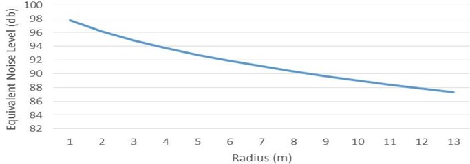
These sound levels that show on illustration (Fig. 1), calculated for radius (3) that is measured from the centerline of road. For radius affection in noise level, different method was conducted. Volume and speed were assumed as constant values in model. The values were selected from Jul-23 that were taken before and sound level was calculated with different amount of “”. The illustration (Fig. 2), shows the sound level changes in different distances.
As it is obvious, when distance increases, sound level will be decreased. As distance increases, sound level depends less than it was in closer distance.
Fig. 1Equivalent noise level variations for one month in studied highway
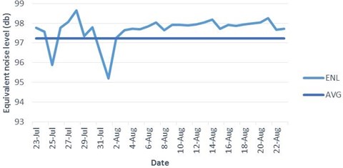
Fig. 2Equivalent noise level variations in different distances from source
4. Conclusions
In this research, the most important traffic parameters that effect on noise pollution consist of average speed of vehicles and traffic volume of road [13]. Average speed effects on noise pollution due to rolling speed of tires. When tires rolling in high speed, they have less friction with pavement. In conclusion, in high speed, vehicles produce less noise than when they are in low speed. Many studies have been conducted in various areas to understand noise pollution effects and all of them reached the same result, for instance, MAP TA Phut port and Bangkok Highway [14]. In result, in rush hours, when the volume of vehicles is in its most and their speed in low, noise pollution of the area increases. But when the road in clear and speed in high and volume is low, sound level reaches its lowest value. The illustration below, shows sound level calculations of one month in summer for Azadegan highway in Tehran. Average sound level of this highway is 97.23 (dB) that illustrated with one straight line.
References
-
Bezan A., et al. Noise pollution a serious threat for human health. 6th Civil Engineer International Congress in Tehran, 2011.
-
Roschke P. Roadway Soundwall and Sound-Reducing Modules Used Therein. US5965852 A, USA, 1999.
-
Transportation Research. Porous Asphalt. 86/RRRI/228, Department of Transportation, Tehran.
-
UNHCS Design Specifications for Porous Asphalt Pavement. University of New Hampshire, New Hampshire, 2009.
-
Makarewicz R. The annual average sound level of road traffic noise estimated from the speed-flow diagram. Applied Acoustics, Vol. 74, Issue 5, 2013, p. 669-674.
-
Rahmani S., Mousavi S. M. Modeling of road-traffic noise with the use of genetic algorithm. Applied Soft Computing, Vol. 11, Issue 1, 2011, p. 1008-1013.
-
Li B. A GIS based road traffic noise prediction model. Applied Acoustics, Vol. 63, Issue 6, 2002, p. 679-691.
-
Ranjbar H., et al. Map modeling of noise pollution with use of SMM1 standard model. 20th International Congress of Geomathic, Tehran, 2013.
-
Seshagiri R. A model for computing environmental noise levels due to motor vehicle traffic in Visakhapatnam City. Applied Acoustics, Vol. 27, Issue 2, 1989, p. 129-136.
-
Phan H., et al. Characteristics of road traffic noise in Hanoi and Ho Chi Minh City. Applied Acoustics, Vol. 71, Issue 5, 2010, p. 479-485.
-
Golmohammadi R., et al. Road traffic noise model. Journal of Research in Health Sciences, Vol. 7, Issue 1, 2007, p. 13-17.
-
Trafficcontrol. Traffic Control Department, 2014, trafficcontrol.tehran.ir.
-
Makarewicz R., Galuszka M. Road traffic noise prediction based on speed-flow diagram. Applied Acoustics, Vol. 72, Issue 4, 2011, p. 190-195.
-
Saffarzadeh M., Rahimi F. Noise Pollution in Transportation Systems. Environment Ministary, Tehran, 2002.
About this article

