Abstract
In this paper, the dynamics of a Bertrand duopoly game with technology innovation have been studied, which contains boundedly rational and naive players. They have been analyzed that the stability of the equilibrium point, the bifurcation and chaotic behavior of the dynamic system. It has been proved that technology innovation has played a very important role in the stability of Nash equilibrium point. Technology innovation can enlarge the stability region of the speed and control the chaos of the dynamic system effectively.
1. Introduction
Cournot game [1] and Bertrand game [2] are the classic models of oligopoly competition. In Cournot game, oligopoly enterprises put the product output as the decision variable and choose the optimal output for high profits. In Bertrand competition, duopoly enterprises play a game based on product differentiation and determine a proper price to obtain the huge profits. In reality, oligopoly enterprises make the output and price decision dynamically and often adjust the decision based on market demand, the decision of competitors, their own production capacity and so on.
In the past, a large number of literatures did the research on dynamic behavior of Cournot and Bertrand game, such as A.A. Elsadany [3], Xiaolong Zhu [4], H. N. Agiza [5], A. K. Naimzada [6], Jixiang Zhang [7], Luciano Fanti [8], Baogui Xin [9] and so on, which involved several adjustment rules: naïve [8, 10, 11], adaptive [5, 12], bounded rational [3, 4, 7, 13, 14] and local monopolistic approximation [3, 14]. Basically, research results of all these papers show that bifurcation and chaos exist in the dynamic system of Cournot and Bertrand game [3-14]. The parameter, adjustment speed of bounded rational player is an important factor which influences the stability of Nash equilibrium point and incurs bifurcation and chaos. What’s more, keeping low adjustment speed can control the chaos.
Previous research conclusions seem unified but not rich. It still lacks studies about the influence of other parameters on the stability of dynamic system. It is well-known that technology innovation plays an important role in economic development. It can enhance the competitive advantage and increase profit of enterprises. Then, can it improve the stability of dynamic systems?
Following the method of Zhang [7] and Agiza [5], this article explores the dynamics of Bertrand duopoly game between boundedly rational and naive players and study the effects of technology innovation on the dynamics of Bertrand model. The paper is structured as follows: In Section 2, a dynamic Bertrand duopoly game model was built which is composed of players that produce heterogeneous products and have different price adjustment rules. In Section 3, the dynamic behaviors and the equilibrium points were studied. The conditions for the existence and local stability of the equilibrium points will be also analyzed. In Section 4, the dynamic system was simulated via many bifurcation figures. The Section 5 drew the conclusion.
2. The model
We consider a Bertrand-type duopoly market where two oligopolies choose different prices for their heterogeneous products. Players can decide the prices according to the adjustment rules.
Let , 1, 2 represents the price of firm at discrete-time periods 0, 1, 2, ..., represents the output. Following Zhang [7], suppose the market demand function of the players is:
where , , , 2, . The parameter measures the degree of substitution of the two products. Large represents big degree of substitution.
Positive parameter is the initial marginal cost of firm . The production cost will be reduced by technological innovation. Let represents the reduction degree of the marginal cost of the firm . is positive correlation with technology innovation investment and can be used to measure the degree of technology innovation. Furthermore, the firm can benefit from another firm’s innovation because technique innovation has externality and spillover effect. Let is the degree of technology spillover. The marginal cost function of the players can be assumed as follows:
where, 0 namely hold.
With these assumptions, the profit of the firm in the single period can be given by:
From the profit maximization by player , the marginal profits in period are obtained as:
Then, the optimal price response function of firm can be given by:
Information in the market usually is incomplete. Supposing players use different expectations to adjust the prices. Following Zhang [7]and Agiza [5], suppose player 1 is boundedly rational [7] and player 2 is naïve [5].
Boundedly rational player 1 makes its price decision based on an estimate of the marginal profit [7]. Namely it decides to increase its price if it has a positive marginal profit, or decreases its price when the marginal profit is negative. Then the dynamical equation of player 1 can be given by:
where is a positive parameter which reflects the speed of price adjustment.
Naive player 2 makes its price decision according to the naive expectations rule [8]. The player 2 decides its prices with his reaction function. Hence the dynamic equation of the naive expectation player 2 can be given by:
With above assumptions, the duopoly game with heterogeneous players is formed from combining Eqs. (6) and (7). Then the dynamical system of the heterogenous players is described as:
3. Nash equilibrium and local stability
In this part the equilibria points of dynamic system will be first studied Eq. (8), and then the stability will be discussed.
The dynamic duopoly game will achieve a Nash Equilibrium at last. The possible equilibrium point of the map Eq. (8) can be obtained as nonnegative solution of the nonlinear algebraic system:
Find that the system (9) is not associated with the parameter . After the calculation of the system it was found that the map has two equilibrium points:
where:
In the traditional economic view, non-negative equilibrium is meaningful. Obviously, is a boundary equilibria (). is the unique Nash equilibrium point and has economic meaning provided that:
where, the above two inequalities are obvious, then Eq. (12) is equivalent to .
In order to study the local stability of equilibrium, the Jacobian matrix of map Eq. (8) should be considered. The matrix form is as follows:
The equilibrium point is stable only when all eigenvalues ( 1, 2) of the Jacobian matrix satisfy 0. According to this theory, the following result about can be received.
Proposition 1. The equilibrium point of system Eq. (8) is a saddle point.
Proof. The Jacobian matrix of has the form:
Its’ eigenvalues are:
For the condition that , , , , are all positive parameters, 1 is workable. Then the equilibrium point is a saddle node. The proof of the proposition is completed.
Next the local stability of the Nash equilibrium point will be studied. The Jacobian matrix of is:
where, the trace of is:
The determinant of is:
The characteristic equation of is:
The discriminant is:
Since 0, the eigenvalues of Nash equilibrium are real.
Necessary and sufficient conditions for local stability of the Nash equilibrium are the Jury’s condition, which is given by:
Since:
Then replace , Eqs. (21) can be simplified as:
(II) is always satisfied.
Since:
(III) is always satisfied.
Then focus on the inequality (I).
Since:
Then replace , . Since, (I) is equivalent to:
From what has been mentioned above, the following conclusion can come out:
Proposition 2. The Nash equilibrium at is stable if and only if the inequality Eq. (24) holds.
Proposition 2 characterizes the stability region in which the Nash equilibrium is local stable. The violation of the inequality Eq. (24) will lead to a flip bifurcation [3].
Noticing that the stability region is associated with and . The propositions can be given about the degree of technology innovation and the degree of technology spillover.
Proposition 3. When , the evolution of price system Eq. (8) is in a stable state and is the Nash equilibrium point. Otherwise, the price evolution is in bifurcation or chaos. Where:
Proof. According to the stability theory of Jury’s condition, the flip bifurcation occurs when 0. Namely:
Then .
So, the system is in stable when , otherwise in bifurcation or chaos.
Proposition 4. When, the evolution of price system Eq. (8) is in a stable state and is the Nash equilibrium point. Otherwise, the price evolution is in bifurcation or chaos. Where:
Proof. According to the stability theory of Jury’s condition, the flip bifurcation occurs when 0. Namely:
Then .
So, the system is in stable when , otherwise in bifurcation or chaos.
From the above description and Proposition, it can be concluded that high technology innovation is beneficial to obtain a steady state and the Nash equilibrium profit. It can expand the stable region and enhance the stability of the product price of market to increase technical innovation.
4. Numerical simulations
The purpose of this part is to illustrate the qualitative behavior of the solutions of the duopoly dynamic system Eq. (8) and provide some numerical evidences to prove above results.
In Fig. 1 ( 5, 1, 0.3, 2, 3, 2, 0.5, 0.32) Nash equilibrium is locally stable approaches to the stable point (3.031, 3.229) for large values of , to be specific, when 0.905. With the reduction of , the Nash equilibrium point becoming instable, period-halving bifurcation and chaos will occur.
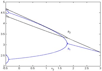
In Fig. 2 ( 5, 1, 0.3, 2, 3, 1, 0.5, 0.32) the Nash equilibrium is locally stable only when 1.769 ( 5, 1, 0.3, 2, 3, 1, 0.5, 0.32). The dynamic system is in bifurcation or chaos if the technology innovation degree is small.
Fig. 1Bifurcation diagram with respect to x1
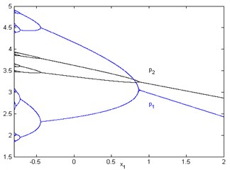
Fig. 2Bifurcation diagram with respect to x2
5. Conclusions
This paper established the price dynamic game model and then analyzed the influence of technology innovation on the equilibrium stability. The results show that technology innovation plays an important role in improving the stability of equilibrium. Specifically, it can enlarge the stability region and make the original bifurcation and chaos change into stability to increase the degree of technology innovation.
References
-
Cournot A. Researches into the Mathematical Principles of the Theory of Wealth. Macmillan, USA, 1897.
-
Bertrand J. Theorie mathematiquede la richesse sociale. Journal des Savants, Vol. 67, 1883, p. 499-508.
-
Elsadany A. A. A dynamic Cournot duopoly model with different strategies. Journal of the Egyptian Mathematical Society, Vol. 23, Issue 1, 2015, p. 56-61.
-
Zhu Xiaolong, Zhu Weidong, Yu Lei Analysis of a nonlinear mixed Cournot game with boundedly rational players. Chaos, Solitons and Fractals, Vol. 59, 2014, p. 82-88.
-
Agiza H. N., Elsadany A. A. Chaotic dynamics in nonlinear duopoly game with heterogeneous players. Applied Mathematics and Computation, Vol. 149, Issue 3, 2004, p. 843-860.
-
Naimzada A. K., Tramontan F. Dynamic properties of a Cournot–Bertrand duopoly game with differentiated products. Economic Modelling, Vol. 29, Issue 4, 2012, p. 1436-1439.
-
Zhang Jixiang, Da Qingli, Wang Yanhua The dynamics of Bertrand model with bounded rationality. Chaos, Solitons and Fractals, Vol. 39, Issue 5, 2009, p. 2048-2055.
-
Luciano Fanti, Luca Gori The dynamics of a differentiated duopoly with quantity competition. Economic Modelling, Vol. 29, Issue 2, 2012, p. 421-427.
-
Xin Baogui, Chen Tong On a master-slave Bertrand game mode. Economic Modelling, Vol. 28, Issue 4, 2011, p. 1864-1870.
-
Bischi G. I., Lamantia F. Nonlinear duopoly games with positive cost externalities due to spillover effects. Chaos, Solitons and Fractals, Vol. 13, Issue 4, 2002, p. 805-822.
-
Kopel M. Simple and complex adjustment dynamics in Cournot duopoly models. Chaos, Solitons and Fractals, Vol. 7, Issue 12, 1996, p. 2031-2048.
-
Elabbasy E. M., Agiza H. N., Elsadany A. A. Analysis of nonlinear triopoly game with heterogeneous players. Computers and Mathematics with Applications, Vol. 57, Issue 3, 2009, p. 488-499.
-
Bischi Gi, Naimzada A., Sbragia L. Oligopoly games with local monopolistic approximation. Journal of Economic Behavior and Organization, Vol. 62, Issue 3, 2007, p. 371-388.
-
Naimzada A., Sbragia L. Oligopoly games with nonlinear demand and cost functions: two boundedly rational adjustment processes. Chaos, Solitons and Fractals, Vol. 29, Issue 3, 2006, p. 707-722.
Cited by
About this article

We wish to thank Hua Zhao and Jianjun Long and some commissions for the research assistance. This study is supported by National Social Science Fund of China (16BGL201), National Social Science Fund of China (14BGL163), Philosophy Social Science Planning Project of Anhui Province (AHSKY2016D14), Research Start-up Fund of Anhui Polytechnic University (2015YQQ004), Youth Research Fund of Anhui Polytechnic University (2016YQ32).
