Abstract
In the paper, the dynamic analysis of a concrete gravity dam was presented. The paper concerns the nonlinear dynamic analysis of an existing concrete dam subjected to a real moderate seismic shock calculated by time history analysis. The linear, elastic, response spectrum analysis was also performed. The dynamic analysis was carried out for 2D and 3D numerical models of the dam. The 2D model represented the middle section of dam’s segment, whereas the 3D model reflected the whole segment. The concrete damage plasticity model (CDP) as a constitutive model of concrete was taking into account. Principal stresses, plastic deformations and degradation of the dam under the shock were evaluated. The results obtained for both models (2D and 3D) were compared. The 3D analysis led to the results revealing material degradation (tensile/compression cracks, stiffness degradation). Such behavior was not obtained for the 2D model.
1. Introduction
The risk evaluation of seismic shock in Poland are currently topic of many studies. The most susceptible structures to seismic tremor are the long or massive objects. This structures like bridges, skyscrapers or dams are very important in terms of economic, urban and safety. The protection against damage or failure of this structures are the key task for civil engineering. There are many dynamic studies about influence of seismic and mining excitation to engineering structures in literature [1-3].
In the paper, the dynamic response analysis of a gravity dam subjected to seismic shock was presented. The gravity dam is typical massive object of which damages may lead to catastrophe. During analysis, the full-time and spectrum analysis were performed. In order to determine damages and stress level under seismic shocks, the concrete damage plasticity model was used. In addition, the two-dimensional and three-dimensional numerical model were prepared. This treatment allows to estimate utility of simplification in numerical model.
2. Geometry of gravity dam and numerical model
The real concrete gravity dam was taking into account during dynamic analysis. The dam is located in Rożnów on the Dunajec river (South Poland). The structure consists of seven delated sections. The high of the dam is about 46 m. The plan dimensions of the segment are 40×20 m. Dilations located between each adjacent segment, protect the structure against excessive strain or stress and provide the independent behavior of segments during seismic events. Hance, only one section of dam was analyzed in the studies.
In order to carry out the dynamic analysis the numerical model must be created. The two kinds of numerical models (2D and 3D) were created. First model, the 2D model represent the middle section of dam’s part. The geometry of section and position of inspection galleries were taking into account. In addition, the mass of the head water was also considering. The structure represented by 2D model was analyzed with a plane strain. The second model, the 3D model represents whole part of dam. 3D model includes the inspection galleries, the crest of dam with parapet walls and also the spillways and sluice ways. The mass of water was also added in 3D model. In both models, the mass of water and also the water pressure were added according to the Westergaard model [4].
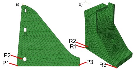
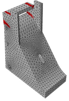
The finite element mesh was fitted based on convergence analysis. The natural frequencies of the structure were tested during convergence analysis. The final mesh for both models were presented in Fig. 1. The total number of finite elements in the 2D model was 607 (Fig. 1(a)), and in the 3D model over 30 000 (Fig. 1(b)).
To represent the more realistic behavior of the dam the advanced material model was applied. The concrete damage plasticity model (CDP) as a constitutive model of concrete was taking into account. The CDP model represents the elastic-plastic behavior of the concrete. Additionally, the typical phenomena for concrete material during cycling load (like tensile and compression damage) were also represented by CDP model. The parameters of the plastic and damage behavior of the concrete were taken from [5]. The elastic parameters were as fallowing: Young modulus 32 GPa, Poisson ratio 0.2, compression strength 24 MPa, tension strength 2.9 MPa.
Fig. 1a) 2D, b) 3D numerical model with a mesh
3. Seismic input data
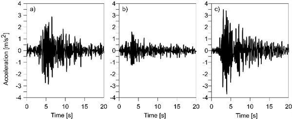
The dynamic analysis was carried out for a moderate seismic shock as a kinematic excitation. The real shock registered in Jarocin (Poland) in 2012 was used. The time history of acceleration in three directions were recorded. The peak ground acceleration in horizontal direction equaled 1.8 mm/s2. For the analysis of moderate shock the value of PGA were scaled up to 3.3 m/s2 and 3.5 m/s2 for horizontal and vertical direction, respectively (see Fig. 2). This value corresponds to the maximum PGA determined for the Central Europe [6]. The dominant frequencies of the shock were located in the range of 3-4 Hz for each direction. The registered accelerations were taken in the studies as the acceleration of the structure supports. The excitation was applying in two directions (NS and vertical) for 2D model and in three directions for 3D model.
Fig. 2Accelerations of seismic shock registered in Jarocin: a) NS, b) WE, c) vertical direction
4. Response spectrum input data
The dynamic analysis was also concerns Response Spectrum Analysis (RSA). During RSA the standard spectral curve was used. The spectral curve form Eurocode 8 was taking into account [7]. The curve parameters were matched for 2nd type of spectrum and ground conditions B. It corresponds, to foundation consisting of very dense sand and magnitude of tremor not greater than 5.5. The used spectral curve was shown in Fig. 3. The value of design ground acceleration was 3.3 m/s2. The RSA was conducted for both numerical models.
Fig. 3Standard spectrum curve used during analysis [7]
![Standard spectrum curve used during analysis [7]](https://static-01.extrica.com/articles/19057/19057-img3.jpg)
5. Results of numerical analysis
The dynamic response analysis of gravity dam to a seismic shock was conducted using ABAQUS Software [5]. The time history analysis (THA) of stresses and also the response spectrum analysis was applied. Because of the anisotropic characteristics of concrete (different tensile and compression strength) the principal stresses were taking into account. This type of stress measure allows to describe both the maximum compression and maximum tension stress. In this study, the results for six representative elements were presented (see Fig. 1). Elements P1-P3 were situated in 2D numerical model and elements R1-R3 in 3D model. All elements were located at the bottom of the dam. Additionally, element P2 was situated on the wall of inside gallery. The location of elements R1-R3 correspond to the elements P1-P3.
Firstly, results for the 2D model were calculated. The stresses obtained from the time history analysis as well as from the response spectrum analysis for the representative elements are shown in Fig. 4.
Fig. 4Principal stresses obtained from time history analysis (black lines) and from response spectrum analysis (red lines) for representative points: a) P1, b) P2, c) P3 for 2D model
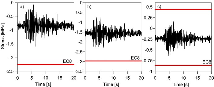
In the Fig. 4(a) the stress in element P1 was presented. It was clearly to see that the stress was below zero for whole analysis time. It shows that element P1 was constantly compressed. In that case the tensile damage dangerous may be ignored. It is worth to mentioned that the compression stress oscillated around constant value. That constant stress came from the dead load and equals about 0.8 MPa. The maximum of compression stress reached 1.6 MPa and appeared in 6 s of shock. It was the time of maximum horizontal peak ground acceleration. The maximum stress was greater than the dead load stress over two times. Comparing the stress from THA and the stress from RSA it can be noticed that the RSA led to more conservative results. The stress obtained during RSA equals 2.2 MPa. It was about 40 % greater than peak stress from THA.
In the Fig. 4(b) the stress in element P2 was presented. The time history of stress in element P2 showed similar relation as in element P1. In element P2 only compression stress occurred. The dead load stress equals 1.5 MPa and the maximum value of stress comes from the seismic shock reached 2.3 MPa. The stress from RSA was much greater than the peak stress from THA. The difference equals 0.7 MPa.
The stress distribution in element P3 (see Fig. 4(c)) represented much complex behavior than in elements P1 and P2. Even though the gravity force induced the compression stress, the compression stress as well as tensile stress occurred during excitation time. The maximum compression stress appeared in 5 s of shock and equal 0.6 MPa. The most dangerous for concrete structure was the tensile stress. Because of the low strength for tensile, even the relatively low tensile stress may result of the cracking of structure. In element P3 the peak tensile stress reached 0.2 MPa. It was 10 % of the strength of concrete. In that case no damages were expected. Next, the comparison of results from THA and RSA were taking into account. The stress obtained during spectrum analysis showed greater value than stress from full time analysis. Both tensile and compression stress were estimated with some excess stress. The stress from RSA were about 0.2 MPa greater than the maximum tensile as well as compression stress from THA.
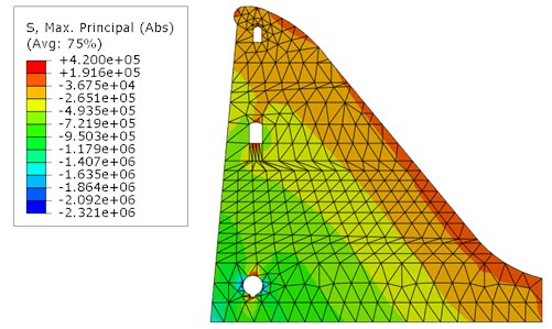
In addition, the map of stress distribution for 2D model were taking into account. The map was presented in Fig. 5. In the Fig. 5 the map of stress in 5 s of shock was shown. It was the time of maximum intensity of seismic excitation and the time when the stress reaches the maximum level. Based on the map it can be noticed that the almost whole structure was compressed. The tensile stress occurred only on the downstream side of structure. The tensile stress concentration appeared also near the hollows (galleries). Maximum tensile stress reached 0.42 MPa. This value was significantly smaller than the tensile strength of concrete material. There was no damage in the dam structure.
Fig. 5Distribution of Maximal Principal Stress for THA for 2D numerical model (in 5 s of shock)
In the next step of dynamic analysis, the stress for 3D model were calculated. Some results of calculation were presented in Fig. 6. The stress obtained during full time analysis were marked with a black line; the stress from spectral analysis were marked with red line. In the Fig. 6 similarly as in previous part of analysis, the principal stress was presented.
In the Fig. 6(a) it can be seen the stress registered in element R1. In this element compression and also tension appeared. The maximum compression stress reached 1.8 MPa while the tension stress 0.9 MPa. That compression stress were over three times greater than the stress from the dead load. Based on the results of spectrum analysis, it can be noticed that the tensile stress reached about 1.9 MPa. It was greater than peak stress calculated by full time analysis. The difference equals 1 MPa. The difference between maximum compression stress obtained during THA and RSA was a little smaller than in case of tension. The value of stress in both analysis differ by 0.8 MPa.
Fig. 6Principal stresses obtained from time history analysis (black lines) and from response spectrum analysis (red lines) for representative points: a) R1, b) R2, c) R3 for 3D model
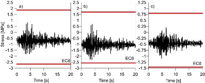
Fig. 6(b) and Fig. 6(c) represent the stress histories in element R2 and R3, respectively. In each case in the elements the compression and tension stress can be observed. The maximum compression stress in element R2 reached 2.25 MPa and in element R3 1.15 MPa. For both elements, stress obtained in RSA were greater than in THA. The difference between stress obtained by various method reach 0.2 MPa for element R2 and 0.5 MPa for element R3. Much bigger differences occurred for tensile stress. Tensile stress in element R2 reached 1.7 MPa for spectrum analysis whereas for full time analysis 0.8 MPa. In element R3 the relationship was similar- peak stress for THA equal 0.25 MPa and for RSA 0.77 MPa. It is worth to mentioned that in each element the tensile stress was not exceed the tensile strength.
The last part of analysis was to compare the results for 2D and 3D model. Because elements P1-P3 correspond in location with elements R1-R3 comparison was possible. Based on Fig. 4 and Fig. 6 it can be seen, that the analysis of 3D model gives greater value of stress than 2D model analysis. For each element, the tension as well as compression stress was greater in 3D model. The biggest different in compression stress can be observed for element P3 and R3. The compression stress varies by 0.5 MPa which was almost 100 %. In the remaining elements, the difference reached 10-20 %. The similar situation can be noticed for tensile stress. For elements P1 and P2 in 2D model the tensile stress did not appeared whereas in 3D model in the same elements the tensile stress reach about 0.8 MPa. It was very important observation because of the vulnerability of concrete to tension.
Fig. 7Distribution of damages after seismic excitation
Additionally, in the 3D model the local damages can be observed. In some elements of construction, the cracks were appeared. The localization of damages was presented on Fig. 7. The red part of structure represented damaged elements. The stiffness of this elements significantly decreased and it was susceptible to subsequent degradation of structure. All of the damaged elements were located in the crown of the dam.
6. Conclusions
The dynamic analysis of gravity dam to a seismic shock, using CDP material model, allow to formulate the fallowing conclusions:
1) The seismic shock influenced the analyzed dam. The maximum expected in Poland, seismic shock caused a significant increase of stress. The stress comes from the dead load was over 2-3 times smaller than the peak stress appeared during seismic excitation. In addition, the seismic tremor generated the tensile stress in structural elements. It is very dangerous in case of a low tensile strength of concrete.
2) Using two different kind of numerical models shows that the 3D model present much better results than 2D model. The stress obtained for 2D model was lower than the stress for 3D model. It leads to underestimation the dynamic response of dam. Some of the phenomenon like damage and failure of some elements occurred during the shock in 3D model only. In 3D model, the seismic shock caused local cracks of structure- it does not appear in 2D model. The calculations with 3D model allow to obtain more safety results.
3) sThe comparison of results obtained from time history analysis and response spectrum analysis indicated that the spectrum method allows to approximate the solution. The stress obtained during spectrum analysis were greater than stress from full time analysis. The difference between results from THA and RSA were about 20-50 %. It was observed for both 2D and 3D model. Because of the stress reserved and the time of calculation, the solution for RSA may be used as a safety estimation of dynamic response.
References
-
Dulinska J., Galuszka A. 3D vs. 2D Modeling of concrete gravity dam subjected to mining tremor. Applied Mechanics and Materials, Vol. 405, Issue 408, 2013, p. 2015-2019.
-
Dunben S., Qingwen R. Seismic damage analysis of concrete gravity dam based on wavelet transform. Shock and Vibration, 2016, https://doi.org/10.1155/2016/6841836.
-
Omidi O., Valliappan S., Lotfi V. Seismic cracking of concrete gravity dams by plastic–damage model using different damping mechanisms. Finite Elements in Analysis and Design, Vol. 63, 2013, p. 80-97.
-
Mays J. R., Roehm L. H. Hydrodynamic pressure in a dam-reservoir system. Computers and Structures, Vol. 40, 1991, p. 281-291.
-
ABAQUS 2012 User Manual V.6.12-2, Dassault Systems Simulia Corp., Providence.
-
Guterch B. Seismicity in Poland in the light of historical records. Przegląd Geologiczny, Vol. 57, Issue 6, 2009, p. 513-520.
-
EN 1998-1, Eurocode 8, Design of Structures for Earthquake Resistance – Part 1: General Rules, Seismic Actions and Rules for Buildings, 2003.
About this article

