Abstract
Because of time-varying, nonlinearity and complexity of the machining process, the traditional PID control has been unable to meet the requirements, which are being high-speed and high-precision. However, an advanced control methods can be a good solution for this kind of control system, a prefect simulation results depends on the accuracy of the modeling process, such models can be used to develop more precise and formalized description of process activities, on modeling process, and now a days a lot of software had been used do this issue. This paper aims to create a milling machine process model using the Simulink modeling method, which use the logic of cutting process as a mathematical terms indicates areal milling machining equations, and give it appropriate processing parameters to ensure the simulating results are comparable, the step response method will be used as good indicator to compare the Model process, using Matlab analysis, first the process will be modelled in the Matlab software to test the step response under various parameters and then compare the results.
1. Introduction
Two major problems in the field of metal cutting are tool wear and tool breakage. Number of schemes, techniques and paradigms have been used for the development of functional decision making systems that would derive a conclusion on machining process conditions, based on sensor signals [1-3]. There are various numbers of modelling methods to predict the machining process from the cutting force effects point of view, such as FEM modelling, modelling geometric ratio of the engagement of the cutting tool, modeling based on the empirical data and modelling based on a specific cutting force [4-6]. Before we can control a system, we must understand in mathematical terms how the system behaves without control [7], to make the design easer it is often to assume there are limited number of transfer function in the design objective. By using the same idea mentioned in many ways, to improve the metal removal rate, online adjusting the feed-rate to achieve the feed control and considering that in actual cutting process of high speed milling, other consideration, due the change of cutting parameters, the dynamic characteristics of the machine tool and other factor, make the cutting process is highly nonlinear [8], also, the problem of time-varying and uncertainly, therefore, the traditional milling machining modeling method is difficult to obtain the ideal effect. Software process models often represent a networked sequence of activities [9], Simulink is a good tool to represent the function that’s needed to make feedback control works. One of the main advantage of Simulink is the ability to model a nonlinear systems, witch a transfer function is unable to do, another advantage, is ability to take the initial conditions. Such an advantages could therefore serve as abases for directing the model process according to the logic of the cutting process mathematical terms.
The paper has the main objective of introducing and explaining the concepts that characterize the system model, through the step response analysis. In addition, Linear Discrete Process Machining Model and Nonlinear process model are introduced and discussed through a real milling cutting parameters. The main idea of this model using the Fig. 1 contents.
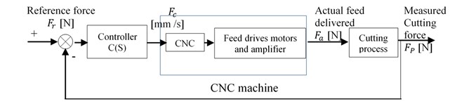
A general block diagram of typical control system is shown in Fig. 1. The input to the system is reference force or desired level of the maximum cutting forces. The actual cutting forces are measured via sensor mounted in the table or in the spindle. The CNC unit sends voltage to the feed drives motor, which move the table at an actual feed velocity of [mm/s]. Because machine tool drive control servos are tuned to be over damp with zero overshoot, they can approximated to have first order dynamic with average time constant.
Fig. 1Block diagram of control system in machining
2. Milling machine process modeling and analysis
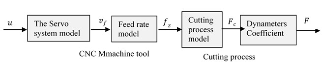
In general, the process model, using the servo mechanism controller is shown in Fig. 2.
Fig. 2Milling machining process model block diagram
2.1. The servo process model
The basic form of a DC servo system is made by an electronic motor [10]. According to the mechanism of the milling model system, [V] and [mm/sec] are the input and output of the servo, they are represented by a second order system:
where, [mm/V’s], [rad/s] and are the servo gain, natural frequency, and damping ratio in sequences.
2.2. Discrete transfer function of the milling process system
As explained in Fig. 1, the machine tool control drive system can be approximated by first continuous system:
where the fa and fc are the actual output and command input values of the feed speed in (mm/s), the feed or chip load per revolution can be founded by [mm/rev] explained in Fig. 3:
where [teeth] is number of teeth on the milling cutter and [rev/s] is the spindle speed.
The cutting force does not change instantly with the feed, it is well known that cutting forces are directly proportional to the chip area behavior [11-13]. A simplified orthogonal cutting force has been introduced in [14] to model the dynamics of the forces in the cutting process:
where [N], (N/mm2), (mm) and are the cutting force, cutting constant, the depth of cut and indexed to the exponent of the specific, respectively, and the process can be approximated to have first-order dynamics as follows:
where is the time constant. The measured cutting force [N], which is orthogonal and proportional to the tangential force can be described by and the process can be approximated to have first-order dynamics as follows:
where, is the dynamometer conversion factor and is the response time parameters of the dynamometer.
3. Types of processing models we can get from the above and analysis
3.1. Linear continuous process model
The process model, can be expresses as a second order transfer function formula:
where, is the total gain of the machining process.
3.2. Linear discrete process machining model
Because of the machining process is controlled at spindle period , the zero-order hold equivalent of is considered:
where is the spindle rotation counter, is forward shift operator and the discrete process parameters (, , , ) depend on the work piece geometry. Assume the milling process transfer function is shown in Table 1.
Table 1Milling process transfer function
Axial cutting depth / mm | Damming ratio | Natural frequency / (rad/sec) | The system gain / (N/V) |
1.91 | 0.1 | 2.3 | 128 |
2.54 | 0.6 | 2.89 | 142 |
3.81 | 0.9 | 2.97 | 206 |
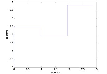
By consider the sampling period time of the model is 0.05 s, and is sampling frequency.
Fig. 3Variation rule of axial cutting depth with time
3.3. Nonlinear machining process model
In a practical servo system there will be additional components of the model witch are important. The most important nonlinearities are the saturation voltage of the motor drive amplifier, the headband in the amplifier, the-called coulomb friction in the rotating mechanical components and hysteresis (backlash) in any gearboxes that might between the motor and the load:
For a nonlinear machining process, the variable gain represent the first-order dynamic system.
Table 2Machining process model parameters
The model | Spindle speed (mm/min) | The feed rate (mm/min) | Back engagement / mm | Axial cutting depth / mm | The Gain / N·s/min | |
G1 | 955 | 380 | 33.8 | 3.2 | 6360 | –5 |
G2 | 955 | 250 | 33.8 | 6.4 | 8586 | –2.8 |
G3 | 955 | 250 | 33.8 | 3.2 | 7473 | –4 |
G4 | 1448 | 890 | 33.8 | 0.75 | 4725 | –3.2 |
G5 | 1448 | 890 | 25 | 1.5 | 7723 | –2.6 |
G6 | 1448 | 1780 | 25 | 2.5 | 6814 | –5.5 |
The process model can be obtained by combining Eq. (8) and Eq. (9).
Eq. (10), represent the system model, in the third- order system. Due to the pole where, –150, when sampling period is 0.02 s, combining Eq. (8) and Eq. (9) can be simplified to:
In the following formula, is the total gain of the machining process. Where the time delay is too much smaller than the time constant . Since the time is small, it can be neglected and the design can be based on the second order model:
In addition, the cutting force does not only has a non-linear relationship with the feed-rate , but also it has a non-linear relationship with back knife as:
In the above formula, is the Exponent, 1, in the milling process 1.4, Eq. (13) will appear as:
4. Milling machine process design model
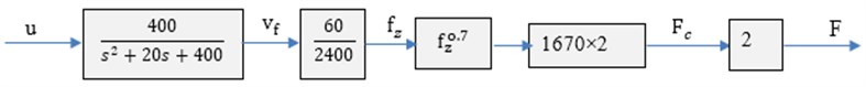
To facilitate the theoretical analysis, assume that, the milling machine is a linear continuous system. By using the model Fig. 4 and give it a real input parameters: 600 [rev/min], 1760 [N/mm2], 1 mm/ (V.s), 2 mm, 4 teeth, 0.5, 0.7 N/mm2, 2 N/mm2 and 20 rad/sec.
Fig. 4Milling machine model
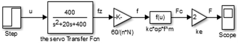
4.1. Establishment of the model in Matlab/Simulink
The established Simulink model shown in Fig. 9, where the simulation parameters mentioned in the above Fig. 4.
Fig. 5The Simulink model of the milling machine controlled system
4.2. Simulation analysis of the milling process in Matlab
To ensure the model correct and comparable, a method using Mat lab code has been developed to test the step response of the established model under various parameters. Parameters MATLAB code had been used to find out the impact of the exponent of the specific m, damping ratio and natural frequency.
4.3. Comparing the final simulation results
When using the same parameters, the step response of all models are the same, which indicate the model is correct and comparable
5. Conclusions
Milling machine model is built in Matlab/Simulink, through the analytical method using linear and nonlinear process. Cutting process is non-linear and the process model varies according to the axial cutting depth, spindle speed, work-piece and cutter shape material, with time. For the model, the discrete transfer- function will be different when the sampling period is different. In addition, the actual process is much more complex than the theory, which cannot able to find the appropriate mathematical model expression to express the process model. Using Matlab/Simulink is can gives more options to change the parameters and simulate additional results, also it is easy to add an advanced controller method to the model.
References
-
Chryssolouris G., Domroese M. An experimental study of strategies for integrating sensor information in machining. CIRP Annals, Vol. 38, Issue 1, 1989, p. 425-428.
-
Chryssolouris G., Domroese M., Zsoldos L. A decision-making strategy for machining control. CIRP Annals, Vol. 39, Issue 1, 1990, p. 501-504.
-
Chryssolouris G., Guillot M., A comparison of statistical and AI approaches to the selection of process parameters in intelligent machining. Journal of Engineering for Industry, Vol. 112, 1990, p. 122-134.
-
Tlusty J. Manufacturing Processes and Equipment. 1st Edition, Upper Saddle River, Prentice-Hall, NJ, 2000.
-
Lasitzhan L. G. Mechanical Vibrations and Industrial Noise Control. Prentice-Hall of India Pvt. Ltd, 2013.
-
Alok Sinha Vibration of Mechanical System. Cambridge University Press, 2012.
-
Crandall S. H., Dahl N. C., Lardner T. J. An Introduction to Mechanics of Solids. Mcgraw-Hill, New York, 1999.
-
Huang Y., Yuan J. High speed constant force milling based on fuzzy controller and BP neural network. International Journal of Control and Automation, Vol. 7, Issue 5, 2014, p. 143-152.
-
Scacchji W. Process Models in Software Engineering. Encyclopedia of Software Engineering, 2011.
-
Elke L. Servo Control Systems 1: Dc Servo Mechanisms. White Paper, Control Systems Principles.
-
Tlusty Ed. J. Manufacturing Processes and Equipment. Prentice Hall, Upper Saddle River, NJ, 2002.
-
Armarego E. J., Epp C. J. An investigation of zero helix peripheral up-milling. International Journal of Machine Tool Design and Research, Vol. 10, Issue 2, 1970, p. 273-291.
-
Oenigsberger F., Sabberwal A. J. P. An investigation into the cutting force pulsations during milling operations. International Journal of Machine Tool Design and Research, Vol. 1, 1961, p. 15-33.
-
Saglam H., Suleyman Y., Unsacar F. The effect of tool geometry and cutting speed on main cutting force and tool tip temperature. Materials and Design, Vol. 28, Issue 1, 2007, p. 101-111.
About this article

This paper is funded by the International Exchange Program of Harbin Engineering University for Innovation-oriented Talents Cultivation.
