Abstract
This paper describes the application of the coordinate transformation matrices into the multi-degree of freedom vibration control. An example with an aluminum beam supported by dual actuators is used to derive how to create both the input transformation matrix and the output transformation matrix. In order to achieve the synchronous movement of the dual actuators, the direct actuator control test and 2DOF control test have been performed. By comparing with the results of the direct actuator control test without using the transformation matrix, the 2DOF control test proves that the transformation matrix is a powerful tool for a significant improvement in test control accuracy.
1. Background
In the field of the environmental vibration tests, Multi-Degree of Freedom vibration test system is able to simulate the dynamic environment more realistically and expose the defects of the large complicated structures more efficiently than by using the single axis excitation. The Multi-DOF vibration test technology has been greatly developed since the 1960s. In recent days, it has been widely used in many areas including the seismic simulation, automobile industry, aerospace, etc. [1-3].
2. The introduction of transformation matrices
Often during the multiple actuator tests, the question arises as to how to arrange the actuators for driving the fixture and how to arrange the transducers for measuring the resulting motion. If more than just linear measurements are required, such as rotations and bending, then a matrix is needed to transform the linear measurements into Degrees of Freedom – the rotations and bending. This matrix is called The Coordinate Transformation Matrix which is determined by the geometry of transducers and actuators [4].
Fig. 1Location of transformation matrices
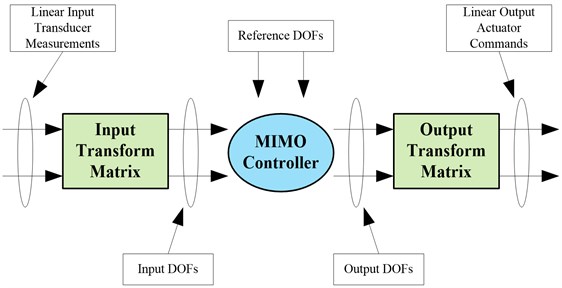
The transformation matrix is usually integrated within the MIMO controller software. However, the transformation matrix can also be located outside of a MIMO control system.
There are two transformation matrices needed. One is at the input to the MIMO Controller and the other is on the output from the MIMO Controller. It is shown in Fig. 1 where the two coordinate Transformation Matrices are located.
The Input Transformation Matrix relates the Linear Input Transducer measurements, sometimes called system response, to the Input Degree of Freedom:
The Output Transformation Matrix relates the Linear Output Actuator commands to the Output Degrees of Freedom:
3. Creating transformation matrices
It is shown in Fig. 2 that an example of symmetric pairs uses a beam with two accelerometer type transducers and located near the ends of the beam. The accelerometers are at a distance from the center of rotation.
Fig. 2Two-dimensional transducer geometry
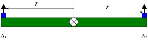
For translation of the beam, both accelerometers must move in the same direction and we take their arithmetic average:
For rotation of the beam, both accelerometers must move in opposite directions. We still take the average but with opposite signs since the signals received from the accelerometers will have opposite signs if there is rotation. In addition, linear acceleration in units of g’s must be converted to angular acceleration in units of radian/sec2. Therefore, both the gravitational constant and the moment arm from the center of rotation are needed:
Converting both equations to matrix form:
Then the input coordinate transformation matrix of this beam example is shown as following:
The same inspection technique can be used to create the output transformation matrix.
For example, suppose we had the same beam as above supported by two actuators. We have two DOF signals, namely translation and rotation from the MIMO Controller and we wish to convert them into actuator signals and .
Fig. 3Two-dimensional actuator geometry
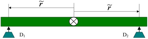
By using the method of creating input transformation matrix, the Linear Output Actuator commands and the Output Degrees of Freedom can be related with the following equation:
But now, the matrix inverse must be used to solve for the actuator signal and :
Finally, the Output Degrees of Freedom and the Linear Output Actuator Commands can be related with the following equation:
Then the output coordinate transformation matrix of this beam example is shown as following:
4. Test setup and validation
4.1. Test system introduction
It is shown in Fig. 4 that the actual dual excitation system consists of a beam and a pair of actuators. The beam is 0.5 meters long, which is made of aluminum. Two 20 N actuators support the beam near the end of it. Also, two accelerometers are located above the actuators. The test requires both of the two actuators move synchronously.
The reference for the test shown in Table 1.
Fig. 4Two-dimensional actuator test system
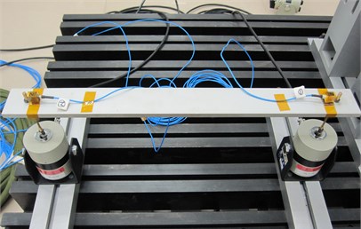
Table 1The reference for the dual actuator test
Element of the reference | Auto power density | Cross power density | |
Coherence | Phase difference | ||
[200-300] +15 dB/Oct [300-500] 1.0×10⁻³ g2/Hz [500-800] –20 dB/Oct | – | ||
– | 0.99 | 0° | |
– | []* | ||
[200-300] +15 dB/Oct [300-500] 1.0×10⁻³ g2/Hz [500-800] –20 dB/Oct | / | ||
4.2. Test and analysis
In order to compare the synchronous control accuracy of this dual actuator system, both the direct square control test and 2DOF control test have been performed. The test results of the two group test will be analyzed in detail as following [5-8].
4.2.1. Direct actuator control
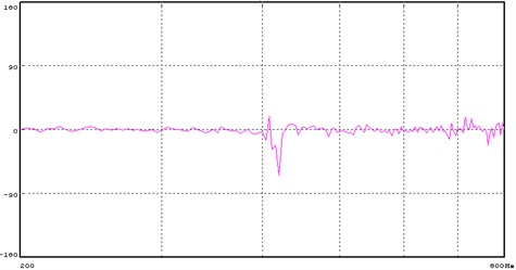
The Direct Actuator Control method will directly control the response of the two accelerometers. Each of the 2 control PSD’s was specified to be the same. Control Phase was set to 0° and the Control Coherence specified as 0.99. Fig. 5 shows the typical control for the 2 vertical accelerometers mounted near the attachment points of the beam and actuators. It should be noted that the two PSD traces nearly overlay each other. Fig. 6 and Fig. 7 shows the coherence and phase difference between the two control points. Note that the coherence reaches about 0.774 at the frequency of 420 Hz, the first resonant frequency of the beam where the phase difference reaches 64.8°, which is the largest one within the whole test frequency band.
Fig. 5Two control results for direct square control
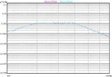
Fig. 6Control coherence for direct square control
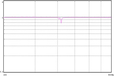
Fig. 7Control phase difference for direct square MIMO control
4.2.2. Two DOF Control
In the second case the same two actuators and control accelerometers were used. However, in this case a Transformation Matrix was used to create virtual controls for translation and rotation motion. The input and output transformation matrices are shown as follows:
The reference PSD for the translation was set the same as the Director Actuator Control Method. But the reference PSD for the rotation was set at a much lower level than the translation. The reason for defining a very low level of rotation is to encourage the translation while suppressing the rotation as much as possible. In this case, the shape of the rotation remains the same as translation but the level of the rotation PSD is at –40 dB of the translation, namely 1.0×10⁻⁷ g2/Hz. Also for this test the Phase between the 2 Control vectors was set to 0° and the Coherence was set to 0.
Fig. 8Control of translation for 2 DOF control
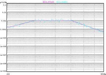
Fig. 9Suppression of roll motion for 2 DOF control
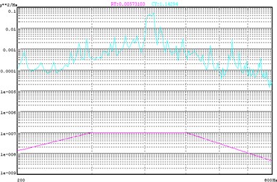
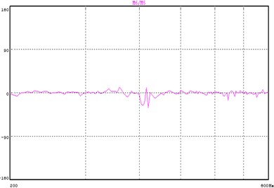
Fig. 8 and Fig. 9 shows the response of the translation degree of freedom and rotation degree of freedom respectively. Note that the translation response nearly overlay the reference of the translation while the rotation response is much higher than the reference. Fig. 10 and Fig. 11 shows the coherence and phase difference between the 2 control points. By comparing this with the results of the Direct Square Control, we can see that at the resonant frequency, the coherence increases from 0.774 to 0.869 while the phase difference decreases from 64.8° to 31.3°. The control effects were greatly improved over the whole test frequency range. It is obvious that by using the 2DOF Transformation matrix to control translation motion and reduce rotation motion, we actually achieve a pure translation of the beam.
Fig. 10Input coherence for 2 DOF control
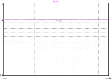
Fig. 11Input phase difference for 2 DOF control
5. Conclusions
The transformation of signals from control transducers into control vectors is a very powerful technique. This newfound transformation flexibility has also created an opportunity to extend the concept to the control of tables, plates and fixtures that may normally exhibit severe torsional responses within the test frequency range. By using transformation matrices derived from the physical system geometry and control transducer placement, a significant improvement in test control accuracy can be perfectly achieved.
References
-
Keller T., Underwood M. A. An application of MIMO techniques to satellite testing. Proceedings: Institute of Environmental Sciences and Technology, USA, 2001.
-
Underwood M. A. Multi-exciter testing applications: theory and practice. Proceedings – Institute of Environmental Sciences and Technology, Anaheim, CA, 2002, p. 1-10.
-
Norman Fitz-Coy, Hale Fitz-Coy, Michael T. On the use of linear accelerometers in 6-DOF laboratory motion replication: a unified time-domain analysis. Proceedings of the 76th Shock and Vibration Symposium, 2005.
-
Underwood Marcos A., Keller Tony Applying coordinate transformations to multi degree of freedom shaker control. Proceedings of the 74th Shock and Vibration Symposium, San Diego, CA, 2003.
-
Underwood M. A., Keller T. Understanding and using the spectral density matrix. Proceedings of the 76th Shock and Vibration Symposium, Destin, Florida, 2005, p. 1-16.
-
Smallwood D. O. Random Vibration testing of a single test item with a multiple input control system. Proceedings of Institute of Environmental Sciences, USA, Dallas, 1982, p. 42-49.
-
Smallwood D. O. Multiple shaker random control with cross coupling. Proceedings of the IES, 1978, p. 341-347.
-
Peeters B., Debille J. MIMO random vibration qualification testing: algorithm and practical experiments. Proceedings of ESTECH 2002, Anaheim, CA, USA, 2002, p. 1-12.
About this article
