Abstract
Model based filtering is fast becoming a key instrument for maintenance and condition monitoring of railway vehicles. This study presents the use of linear Kalman filtering scheme to identify vertical secondary suspension of a railway vehicle by using the vertical vibrations of a vehicle due to vertical track irregularities. As well as the use of linear Kalman filtering scheme, a weighted least squares estimation is used to identify vertical secondary spring coefficient as a parameter by using residuals of the filter. In this investigation, a 7 degree of freedom dynamic model of ERRI B176 benchmark vehicle is considered. Unlike previous studies, to the authors’ knowledge, this research provides the simplest estimation scheme for identification of secondary vertical spring parameter and can be used to achieve a cost-effective condition based maintenance for railway vehicles.
1. Introduction
For mechanical vehicle vibrations, ideal theoretical model generation is a tough job since the physical character is unpredictable due to imperfections between bodies and the environment. Optimization of system parameters like damping factor and stiffness constants needs further investigation under random theory [1]. Even after this investigation, changes may occur in these constants due to operating conditions. Therefore, for safe operation and passenger comfort, these constants should be monitored continuously without waiting a calendar based maintenance schedule.
Online condition monitoring and parameter estimation for railway vehicles are not new concepts. In [2], such a condition monitoring scheme to detect suspension faults based on evaluating cross correlations between the measurements from bogie mounted inertial sensors is proposed. Another investigation [3] is provided by the use of extended Kalman filtering and unscented Kalman filtering to identify suspension parameters based on the vertical dynamic model of a railway vehicle similar to present study.
As well as studies which examine identification of secondary vertical suspension, there exist studies which focus on estimating lateral suspension by interpreting the lateral vibrations of a vehicle due to track irregularities. In [4, 5], the use of Rao-Blackwellised particle filter, which is a filtering technique based on marginalization of a Kalman filter with a particle filter, is reported for estimating secondary lateral and anti-yaw damper. The drawback of such scheme is that particle filters need excessive computation power. In [6], a computationally efficient estimation scheme, which is based on extended Kalman filter, is given. In [6], measurement vector only contains the inertial measurements (accelerometers and gyroscopes). Mounting and placement of such sensors for condition monitoring purposes are presented in [7].
To the authors’ knowledge, this research provides the simplest estimation scheme for identification of secondary vertical springs in related literature. Unlike previous related studies, present study considers the linear Kalman filter and a weighted least squares estimation scheme for identification of secondary vertical springs. A specific advantage of this estimation scheme is that measurements of deformations (i.e. displacements) of suspensions are not required as they are assumed in [3]. Only the inertial measurements are sufficient to identify secondary lateral springs.
2. Dynamic model of the vehicle
Details of 7 degrees of freedom dynamic model, considered hereby, can be found in chapter II.5 of [8]. However, the parameters of the vehicle are selected differently from the parameters indicated in [8]. The parameters are based on ERRI B176 benchmark vehicle given in [9] and related parameters can be found in Table 1. Furthermore, an illustration of the vehicle model is given in Fig. 1.
Table 1Vehicle parameters
Parameter | Definition | Value |
Mass of the coach | 32000 kg | |
Mass of the bogie | 2615 kg | |
Stiffness of the secondary spring | 430×103 N/m | |
Stiffness of the primary spring | 122×104 N/m | |
Damping coefficient of secondary suspension | 20×103 Ns/m | |
Damping coefficient of primary suspension | 4×10³ Ns/m | |
Moment of inertia of the coach around z axis | 197×104 kgm2 | |
Moment of inertia of the coach around x axis | 56800 kgm2 | |
Moment of inertia of the bogie around x axis | 1722 kgm2 | |
Lateral semi spacing of secondary suspension | 1 m | |
Lateral semi spacing of primary suspension | 1 m | |
Longitudinal semi spacing of secondary suspension | 9.5 m | |
Longitudinal semi spacing of secondary suspension | 9.5 m | |
Velocity of the vehicle | 20 m/s |
Fig. 1Illustration of the vehicle model
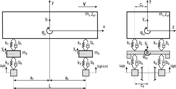
The dynamical model considered in this study is linearized around the operating state and state is given as:
Equations of motions can be presented as:
Definitions of the matrices , , , , can be found in appendix of [8]. is the vector of vertical track irregularities of the left and right side and is the velocity of the vertical track irregularities. For simple numerical calculations, Eq. (2) is written as a first order differential equation as:
In Eq. (3) is defined as:
3. Estimation model, Kalman filter and parameter estimation scheme
For estimation purposes Eq. (3) can be written in continuous time state space form as:
In Eq. 5, represents the states and represents the measurements. Furthermore, represents the inverse of the fist matrix given in Eq. (3) and is the second matrix given in Eq. 3. and are Gaussian process and measurement noises, respectively. In this study, unlike the measurement vector given in [3], which includes the measurements of deformations of suspensions; it is assumed that the measurements are simply taken from low cost inertial sensors (accelerometers and gyros). Mounting and placement of such sensors are reported in [7], as previously stated. Measurement vector can be given as:
For practical purposes, continuous time system given in state space for in Eq. 5 can be written in discrete form as:
The analogy between Eq. (5) and Eq. (6) can be easily seen. In Eq. (7), again represents the states. Definitions of matrices , and can be found in section 8.2 of [10]. Furthermore, , can also be obtained by using the same formalism given in [10]. After discretization of the system, a discrete time Kalman filter can be applied. Time update equations for states and covariance can be given as:
Additionally, measurement update equations can be given as:
In this research, a concurrent state estimation, which time update and measurement update occur simultaneously, is considered. Therefore, for covariance estimation only a posteriori covariance estimate is calculated given in Eq. (9). Discretization step size is 10 milliseconds. In this work, vertical track irregularity information is provided by the measurements from a 3 km track section between Choceň-Dobřikov, Czech Republic.
In [11], it is stated that in parameter estimation aim is to find optimal parameter which give the best fit. This fit is maintained by the minimization of cost function, generally. To determine the cost function, a weighted least squares approach is considered in this investigation. Cost function can be given as:
where is the weighting parameter and is the residual. Hereby, weight vector is determined by simulations. It has been observed that most influential residuals are vertical acceleration and roll rate of the body of the coach. Therefore, these two residuals have the 70 % of the weight and other residuals have the rest of the weight equally. In simple form parameter estimation is done by:
where is a parameter defined to interpret sum of residuals and it is equal to 1.5×10⁶. This parameter is determined by using the simulation results.
4. Simulations and estimation results
Firstly, for model validation, a step input test is investigated. In this test, a 1 mm vertical track irregularity is applied to both bogies after 1 second. It can be seen in Fig. 2 that both response of coach and 2nd bogie converge to the step input value.
Fig. 2Step response of the considered model
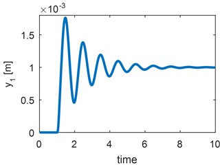
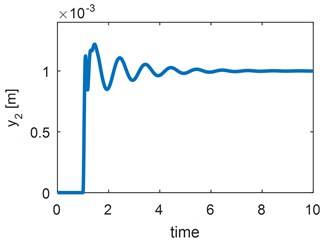
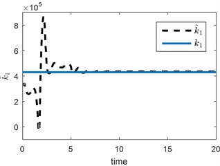
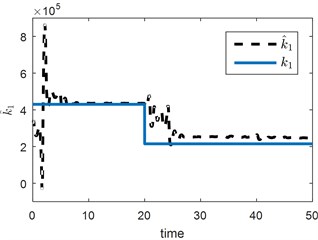
Fig. 3Vertical suspension estimation results for a) static and b) step change tests
a)
b)
The selection of initial covariance matrix is intuitive, whereas process and measurement noise matrices depend on how model represents the physical system and the statistical properties of the used sensors, respectively. Here, initial covariance matrix is selected as a diagonal matrix having the same size of state vector and each diagonal is equal to 0.01. Process noise matrix is selected similar to initial covariance matrix that has the same size of state vector and each diagonal is equal to 0.001. Measurement noise matrix is selected as a diagonal matrix having same size of measurement vector and each diagonal is equal to 1. Firstly, a static estimation scenario is presented. The value of is given in Table 1. In estimation scenario, it is assumed that initial guess of the parameter estimate is equal to 330×103 N/m. It can be clearly seen in Fig. 3 that parameter estimate converges to real value. In the second estimation scenario, with same initial condition selection as in first scenario, it is assumed that at 20 seconds a malfunction occurs and real value of the vertical secondary suspension decreases to the 50 %. Even under these circumstance estimation scheme is promising and sufficient to detect a change in vertical suspension.
5. Conclusions
Condition based monitoring frameworks are challenging to achieve due to the requirement of huge amount of sensors and maintaining their calibration and covariance investigation of different system parameters in railway vehicles. In this study, a model based approach with a linear Kalman filtering scheme is employed to identify the vertical secondary suspension of a railway vehicle by using the vertical vibrations of a vehicle due to vertical track irregularities is proposed. To the authors’ knowledge, this research provides the simplest estimation scheme for identification of secondary vertical springs. Simulation results, considering static and step change tests, are considered to be promising to determine vertical secondary suspension of a railway vehicle. This cost-friendly model based filtering scheme can be used for condition monitoring of secondary suspension instead of calendar based maintenance.
References
-
Yıldıdım Ş., Uzmay İ. Neural network applications to vehicle’s vibration analysis. Mechanism and Machine Theory, Vol. 38, Issue 1, 2003, p. 27-41.
-
Mei T. X., Ding X. J. Condition monitoring of rail vehicle suspensions based on changes in system dynamic interactions. Vehicle System Dynamics, Vol. 47, Issue 9, 2009, p. 1167-1181.
-
Xu B., Zhang J., Guan X. Estimation of the parameters of a railway vehicle suspension using model-based filters with uncertainties. Proceedings of the Institution of Mechanical Engineers, Part F: Journal of Rail and Rapid Transit, Vol. 229, Issue 7, 2015, p. 785-797.
-
Li P., Goodall R., Kadirkamanathan V. Estimation of parameters in a linear state space model using a Rao-Blackwellised particle filter. IEE Proceedings – Control Theory and Applications, Vol. 151, Issue 6, 2004, p. 727-738.
-
Li P., Goodall R., Weston P., Ling C. S., Goodman C., Roberts C. Estimation of railway vehicle suspension parameters for condition monitoring. Control Engineering Practice, Vol. 15, Issue 1, 2007, p. 43-55.
-
Zhang Z., Xu B., Ma L., Geng S. Parameter estimation of a railway vehicle running bogie using extended Kalman filter. Proceedings of the 33rd Chinese Control Conference, Nanjing, 2014.
-
Ward C. P., Weston P. F., Stewart E. J. C., Li H., Goodall R. M., Roberts C., Mei T. X., Charles G., Dixon R. Condition monitoring opportunities using vehicle-based sensors. Proceedings of the Institution of Mechanical Engineers, Part F: Journal of Rail and Rapid Transit, Vol. 2, Issue 225, 2011, p. 202-218.
-
Gerlici J., Lack T., et al. Transport Means Properties Analysis – Vol. 1. EDIS Publishing House of University of Zilina, Zilina, 2005.
-
Iwnicki S. Manchester benchmarks for rail vehicle simulation. Vehicle System Dynamics, Vol. 30, Issues 3-4, 1998, p. 295-313.
-
Simon D. Optimal State Estimation: Kalman, H Infinity, and Nonlinear Approaches. John Wiley and Sons, 2006.
-
Matzuka B., Aoi M., Attarian A., Tran H. Nonlinear Filtering Methodologies for Parameter Estimation. Department of Mathematics, North Carolina State University, 2012.
About this article
