Abstract
This paper proposes a self-iteration principal component extraction (SIPCE) and direct matrix assembly method for three-dimensional structures. Different from calculating principal components (PCs) by matrix decomposition in traditional principal component analysis (PCA), SIPCE extracts PCs one by one through self-iteration, so SIPCE has lower space-time complexity. Besides that, it avoids singular-value and ill-posed problems of matrix decomposition. The previous method of solving three-dimensional structures is using modal coordinate response back general reversion of least square algorithm, while the new matrix assembly method calculates three-dimensional modal shapes at one time. So, the new matrix assembly method has less calculation error. The numerical simulation results in a cylindrical shell demonstrate that this method can be practically and effectively applied in operational modal analysis (OMA) of three-dimensional structures. The new method is also robust to noise, and has higher identification accuracy and lower space-time consumption than previous method.
1. Introduction
From 1980s, OMA deals with the estimation of modal parameters from vibration data obtained in operational rather than laboratory conditions [1]. It seeks to determine structure’s dynamic characteristics by using vibration response only to overcome the conventional experimental modal analysis (EMA) [2]. Some innovative OMA methods have been proposed and applied to practical engineering in recent years. Han S. et al. applied a PCA and orthogonal decomposition method on OMA, and demonstrated the orthogonality of principal modes [3, 4] for dynamic weakly damped mechanical structures. Poncelet et al. introduced the blind source separation (BSS) and the independent component analysis (ICA) techniques [5, 6]. G. Kerschen focused on the physical interpretation of independent component analysis in structural dynamics “For free and random vibrations of weakly damped structures, a one-to-one relationship between the vibration modes and the ICA modes is demonstrated using the concept of virtual source”. [7]. Bai et al. proposed a new method based on manifold learning termed locally linear embedding (LLE) [8].
Principal components analysis (PCA) is a classic data mining method which is firstly proposed in 1901 [9]. In the early 2000s, Kerschen proposed to apply PCA and Orthogonal decomposition in dynamical characterization and order reduction of mechanical systems [10]. However, the existence, uniqueness, physical significance of OMA has no elaboration and proof. Wang et.al [11] found the one-to-one mapping relationship between the modal shape, modal responds and mix matrix, latent variable. Traditional PCA calculates principal components by eigenvalue decomposition (EVD) and singular-value decomposition (SVD). However, ill-posed and singular-value problems exist in these approaches [12]. Besides that, OMA based on traditional PCA has high time and space complexity when there are many response measurement points and sample times. This paper proposes a SIPCE method for OMA, which avoids the shortcomings above.
As is known to all, engineering structure is three-dimensional in practice. The process of one-dimensional extending to three-dimensional is a challenge that must be conquered by OMA methods when the researches of scientific and technological apply to engineering applications. In 2014, C. Wang et al. built a PCA solution model for three-dimensional structures, and gave a scientific three-dimensional matrix assembly method [13]. However, the PCA model is calculated by EVD and the three-dimensional modal shapes are calculated by reverse matrix substitution, so that method has higher space-time complexity and lower identified accuracy. In 2017, J. Wang et al. proposed to use second-order blind identification to solve three-dimensional model [14], and the matrix assembly method is similar to C. Wang’s method. This paper proposes a new matrix assembly method for complex three-dimensional structures, and uses SIPCE to solve PCA model. With comparing with the previous method, this method has higher identification accuracy and lower time and space complexity.
2. Principal component analysis based operational modal analysis
The data set of physical responses (Symbol “” which is in the upper right corner of matrix expressed matrix transpose) is composed byunrelated unknown latent variables through a linear transformation matrix [15], which is shown in Fig. 1:
Matrix meets condition:
uncorrelated latent variables meets condition:
Fig. 1Description of PCA problem
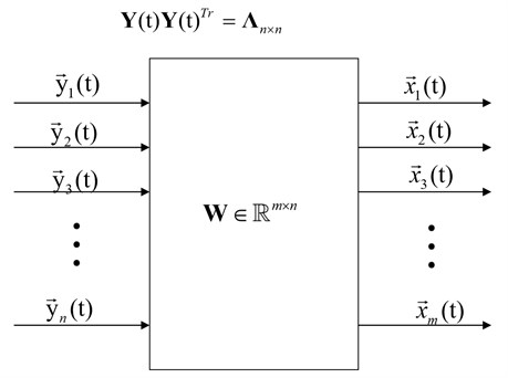
Fig. 1 is the diagram of PCA model. The goal of PCA is to find linear transformation matrix and uncorrelated latent variables only from observed signal .The uncorrelated latent variables are called principal components of observation signal .
According to the theory of structural dynamics, for linear time-invariant (LTI) structures with degrees-of-freedom, the equations of vibration motion in the physical coordinates:
In Eq. (4), matrix is the mass matrix of the LTI structures, matrix denotes the damping matrix of the LTI structure, matrix is the stiffness matrix of the LTI structures, denotes time. Matrix is the time domain random dynamic motivation of the LTI structures, and matrix is the time domain dynamic displacement response of the LTI structures, is the time domain dynamic speed response of the LTI structures. is the time domain dynamic acceleration speed response of the LTI structures.
Viscous damping matrix can’t be orthogonally diagonalized by modal shape, so it can’t be decoupled directly. However, in special cases, matrix could be orthogonally diagonalized. For example, the viscous damping which is proposed by Rayleigh:
In Eq. (5), , denotes as the outside and inside damping constants of the system, for weak damping vibration system, the above model is effective.
Comparing with real mode, the complex mode shapes cannot be represented in real numbers, and this paper mainly focuses on real mode. For real mode, in the modal coordinate, the random vibration response signals of mechanical structures with weak damping can be decomposed into the inner product of modal shapes and modal responses:
where is the output displacement, is the reversible modal shape matrix which composed by independent mode shapes , besides that, is basis-vector matrix in modal coordinate space; and is the modal coordinate matrix which composed by modal response of each mode.
Plugging Eq. (6) into Eq. (4), which transports physical coordinate into modal coordinate:
Simplifying Eq. (7):
Then, Eq. (8) is the modal model, where is modal mass matrix, is modal damping matrix, is modal stiffness matrix:
Based on the vibration theory in Eq. (6)-(14), when the structure’s natural frequencies of each mode are not equal, the modes vectors are orthogonal:
And modal response vectors are independent from each other. Then satisfies:
where is a real positive diagonal matrix.
Natural frequency can be identified by FFT or single degree of freedom (SDOF) fitting techniques from mode coordinate response vector [16]. Fig. 2 is the flowchart of OMA based on PCA modal.
Fig. 2The flowchart of PCA based OMA modal
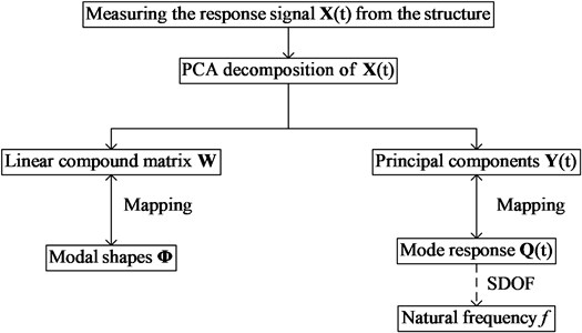
In view of Eq. (1) and Eq. (6), for random vibrations of weakly damped systems, there is a one-to-one mapping between the orthogonal mode matrix and the linear transformation matrix in Eq. (2). Besides that, there is a one-to-one mapping between modal response matrix and the PCs . Therefore, the existence, uniqueness and deterministic of OMA based on PCA algorithm can be proved by PCA decomposition.
3. SIPCE for OMA of three-dimensional structure
3.1. Self-iteration principal component extraction algorithm
The SIPCE algorithm is the improvement of (Nor-linear Iterative Partial Least Squares) NIPALS algorithm [17]. NIPALS gets mutually orthogonal eigenvectors by projecting the high-dimensional data samples to the low-dimensional feature space, then establishing a linear regression relation between eigenvectors [18]. NIPALS model has less Variables, it’s more robust to noise. Since the birth of the NIPALS algorithm, it’s wildly used to calculate PCs, the calculation process is actually equivalent to EVD.
The following are algorithmic steps, a column from the physical responses matrix , 1, 2, …, is chosen. The first principal component vectors is randomly chosen from signal matrix , 1, 2, ..., , and then the first transformation matrix vector is iteratively calculated. As Eq. (17) shows, denotes error matrix, error matrix is updated to calculate the second principal component vectors and the second transformation matrix vector and so on:
Initially setting max iterations times , accuracy threshold , contribution threshold . Assume index denotes the th principal moment, and 1. Setting original error matrix .
Chose the arbitrary column data vector from signal matrix, assume the chosen column is the th column, so vector is chosen from signal matrix , initializing 1.
Calculate : ;
Normalize the vector : ;
Update : ;
Compare the in the step 4) with the in the step 2), define variable , if , go to the step 7); else, 1 and return to the step 2).
Calculate : .
Update the error matrix :
Define the contribution of current mode, if and , 1 and return to the step 2), else go to step 10)
Get the PCs matrix and the linear transformation matrix .
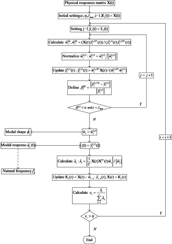
The step 9) is to calculate the oversized contribution rates correspond to the th principal components. So, is the approximate contribution rate, which corresponds to the th principal component. Principal components are extracted by the order of cumulative variance proportion. Contribution rates is the proportional size of the current principal component in all calculated principal components. is contribution threshold, if , stopping iteration, which means the current principal component is not important enough. And the principal components extraction process is complete. Fig. (3) is the flowchart of self-iteration principal component extraction algorithm based on OMA.
Fig. 3 shows the flowchart of self-iteration principal component extraction based OMA algorithm. Variable 1, 2, …, represents the contribution of its corresponding principal components, is the importance index of next principal components, and is a setting threshold value which is used to control the iterations. Therefore, it realizes the principal components extraction.
Table 1The performance comparison of different PCA algorithms
Algorithm | Time complexity | The least space complexity | Algorithm robustness |
PCA based on EVD | High | Singular value problem | |
PCA based on SVD | High | Ill-posed problems | |
SIPCE | , Low | Avoids the ill-posed and singular value problems |
Difference from calculating all modal orders at one time in traditional batch-processing PCA method, SIPCE just extracts several modal orders according to practical need. When there are many response measurement points and sample times, the SIPCE method has obvious advantages in time and space overhead. Besides that, SIPCE calculate modal parameters by iteration, which avoids singular values and ill-posed problem in traditional PCA method, so it always has higher identification accuracy. Table 1 is the comparison between SIPCE and traditional PCA.
Fig. 3The flowchart of self-iteration principal component extraction algorithm based OMA
3.2. Three-dimensional OMA and its differences
Actual engineering structures are three-dimensional. From one-dimensional to three-dimensional, it takes a big step from scientific researches to engineering applications of modal analysis based on a series of blind source separation methods.
The matrix assembles: the vibration matrix of one-dimensional structures is a one-dimensional vector, the proportion of the value of each modal makes sense, but the amplitude of the modal does not make any sense. And the vibration matrix of the three-dimensional structure is combined by three directions , and . Each direction of the scale factor and the modulus ratio should stay the same, otherwise it becomes a one-dimensional vibration mode of three directions, rather than a three-dimensional vibration mode of structures. How to carry out this process is a big challenge.
For continuous three-dimensional structures, in finite element analysis and experimental analysis, the three-dimensional system is discretization to D test points, and the time is discretization to T number of sampling points. The displacement response in time domain can be expressed by modal coordinate approximation [13], both the speed signal and the acceleration signal are also suitable to Eq. (20):
where , are physical responses in three directions, and , , are mode shapes matrixes of , and directions. Matrix is the modal response which contains the information of modal natural frequency. Theoretically infers of three directions are the same.
In three-dimensional modal parameters analysis, modal shape identification is the most important and difficult. Modal shape matrix of one-dimensional structure is a one-dimensional vector, the proportion of each element is crucial. However, the size of element has no practical significance. For modal shape matrix of three-dimensional structure, the three one-dimensional modal shape vectors that in , , direction are arranged in sequence and the proportion of each direction and element must remain fixed. If the proportions are changed, the obtained modal shapes are no longer three-dimensional modal shapes. So, it’s a big change to identify modal shape for three-dimensional structures.
3.3. The Assembled three-dimensional modal shapes
According to the previous method [13], the three directions’ modal coordinate responses are same, so the algorithm decomposes modal response signals in one direction which has the maximum vibration. Then through substitution of into the other two-dimension displacement response signals using Moore-Penrose matrix inverse in Eq. (21), modal shapes of these two dimensional can be identified. And three dimensional modal shapes are assembled:
This paper proposes to assemble three directions’ modal response firstly, assume the assembled matrix is the whole response signal of three-dimensional structure. Then setting and solving the PCA model of the whole response signal, the modal coordinate responses and the three-dimensional modal shapes are calculated directly. The new displacement response in time domain can be freshly expressed by modal coordinate approximation:
where is the assembled modal signal matrix, is the three-dimensional modal shapes and is the modal coordinate response.
The method of least-square inverse matrix substitution firstly gets modal coordinate response of the largest response direction by matrix decomposition, then assume that is the global modal coordinate response to calculate modal shapes of the other two direction. However, the modal coordinate response of the largest response direction is not equal to the global modal coordinate response, there must be error in the final three-dimensional modal shapes. As for direct matrix assemble, it calculates the global modal coordinate response and three-dimensional modal shapes matrix directly by matrix decomposition, thus the new method avoids matrix inversion. In the calculation process, matrix inversion error and Ill-posed problems [20] are inevitable in the calculation, so the new method has higher identification accuracy than the matrix substitution method. Comparing Eq. (21) and Eq. (22), Table 2 is the performance comparison of two methods.
Table 2The performance comparison of different three-dimensional modal assemble algorithms
Method | Least-square matrix substitution | Direct matrix assemble |
Error of matrix inversion | Yes | No |
Ill-posed problems | Yes | No |
Robustness | Sensitive to measurement noise | Insensitive to measurement noise |
3.4. OMA for three-dimensional structure by SIPCE and Direct matrix assemble
In order to identify operational modal parameters of three-dimensional structure, a strategy is adopted as below and the process of OMA for three-dimensional structure is shown in Fig. 4 below.
Fig. 4Process of OMA for three-dimensional structure by SIPCE
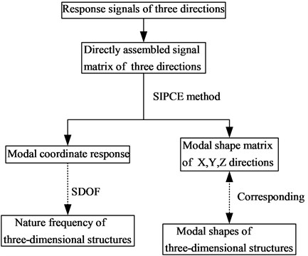
The new method for three-dimensional structure replaces traditional PCA with SIPCE to solve the model. The new method sharply reduces space-time complexity, avoids singular values and ill-posed problem. In addition, the new method calculates modal shapes directly to avoid matrix inversion substitution, thus reducing the identify error. To summarize, SIPCE algorithm and the new modal assemble method can be well used in OMA for three-dimensional structures, and it has higher identification accuracy and lower time-space complexity than previous method.
4. Simulation verification
4.1. Simulation data generation
The simulation data mainly pays attention to the cylindrical shell with two simple supported ends, and the excitation is Gauss white noise. The parameters setting of cylindrical shell is: the thickness is 0.005 m, length is 0.37 m, radius is 0.1825 m, elasticity modulus is 205 GPa, Poisson’s ratio of material is 0.3, density of material is 7850 kg/m3, and mode damping ratios are 0.03, 0.05 and 0.1 respectively.
The cylindrical shell is a continuum structure, and it must be discretized in order to calculate the modal and vibration response of the structure by finite element method. The more the number of discretized units, the more accurate the calculated modal and vibration response. Along the axial cylindrical shell distributes evenly 38 circles, each circle distributes evenly 115 observation spots which are shown in Fig. 5. Thus, the total of observation spots 4370. The uniform white noises excitation is applied at each response point to generate the simulation data. In order to characterize the cylindrical shell structure of the complex three-dimensional mode shape with high accuracy, so many observation spots are chosen in the simulation. Operational modal parameter identification only requires that the number of response points is more than the number of the modal of the structure. So, for a real structure under normal working conditions, SOBI based three-dimensional operational modal parameter identification does not need so many sensors. The sensor points are more than or equal to the number of the modals in three directions of the structure. Of course, the more of the sensor points, the more accurate of the identification mode shapes. At the same time, the sampling frequency is placed at 5120 Hz, and the sampling time is set to 1 s, 5120. The boundary conditions of the cylindrical shell are simply supported at both ends. At last, response signals of three directions are calculated by LMS Virtual.Lab [21] using finite element analysis (FEA). An observation spot is selected randomly, such as the 1118th spot whose response signals of three directions shown in Fig. 6 as below. Response data are divided into two groups: data without measurement noises and data with 5 % Gauss measurement noises.
Fig. 5Three-dimensional picture of the cylindrical shell
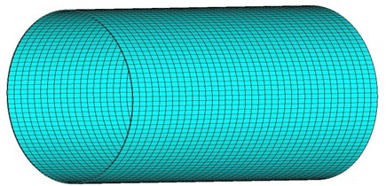
Fig. 6The response signals of three directions
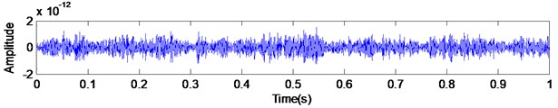
a) Response of direction about the 1118th observation spot

b) Response of direction about the 1118th observation spot
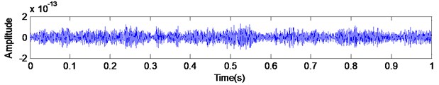
c) Response of direction about the 1118th observation spot
4.2. Evaluation criteria and parameter setting
Theoretical values and FEA values are set as standard, which are calculated under the condition of undamped real modal shape and undamped real modal nature frequency, and PCA algorithm is based on EVD method.
In order to quantitatively compare the modal vibration mode, modal assurance criterion (MAC) is investigated [22], which is an important standard when considering the effectiveness of modal shape identification. It is computed by:
where is the identified shape, represents the real shape, and () represents the inner product of the two vectors. MAC values oscillate between 0 (no coincidence) and 1 (complete coincidence). And the more MAC value is close to 1, the more accurate estimated shape is.
1) Set precision threshold 0.000001;
2) Set maximum number of iteration 100;
3) Set truncation error 0.01;
4)Computer configuration:
Operating system: 64-bit Windows 10,
Manufacturer: HP,
System Type: HP Z240 SFF Workstation,
Processor: Intel(R) Core(TM) i5-6500 CPU @ 3.20 GHz (4 CPUs),
Memory: 8192 MB RAM,
Programing language and environment: MATLAB 2014a.
4.3. Simulation verification results
The modal vibration modes and natural frequencies by the FEA method are used as the real value, show in Fig. 7.
Fig. 7Real mode shapes calculated by FEA
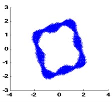
a) The 1th real modal shape
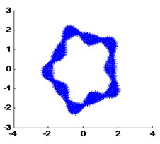
b) The 2th real modal shape
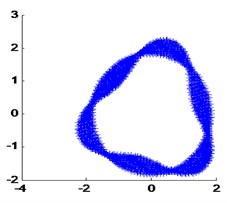
c) The 3th real modal shape
d) The 4th real modal shape
e) The 5th real modal shape
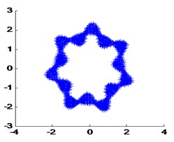
f) The 7th real modal shape
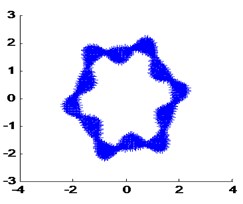
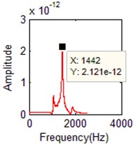
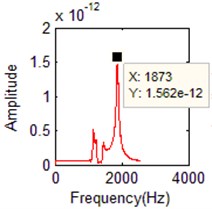
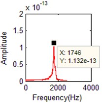
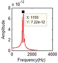
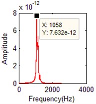
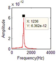
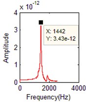
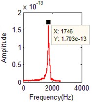
When the damping ratio of the cylindrical shell is 0.03, the mode frequency identified by the purposed algorithm is shown in Fig. 8 below. Table 3 is the identified frequency by the proposed algorithm comparison of real frequency by FEA. Fig. 9 is the identified modal shape, Table 4 is the MAC values of mode shapes.
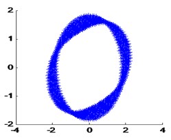
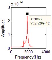
When the damping ratio of the cylindrical shell is 0.03, and the 5 % measure noise is added into the response signals, the mode frequency identified by the purposed algorithm is shown in Fig. 10 below. Table 5 is the identified frequency by the purposed algorithm comparison of real frequency by FEA. Fig. 11 is the identified modal shapes. Table 6 is the MAC values of mode shapes.
Fig. 8The identified mode frequencies when the damping ratio is 0.03
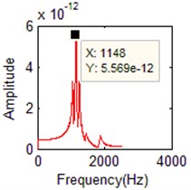
a) FFT of the 1th order
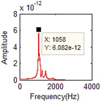
b) FFT of the 2th order
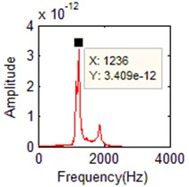
c) FFT of the 3th order
d) FFT of the 4th order
e) FFT of the 5th order
f) FFT of the 6th order
Table 3Comparison of natural frequencies with different method
FEA method | PCA+ Least-square matrix substitution | SIPCE+ Direct matrix assemble | |||||
Orders | Frequency (Hz) | Orders | Frequency (Hz) | Relative error | Orders | Frequency (Hz) | Relative error |
1 | 1054.9 | 2 | 1058 | 0.389 % | 2 | 1058 | 0.294 % |
2 | 1145.7 | 1 | 1150 | 0.026 % | 1 | 1148 | 0.201 % |
3 | 1239.6 | 3 | 1236 | –0.210 % | 3 | 1236 | –0.290 % |
4 | 1441.9 | 4 | 1443 | 0.076 % | 4 | 1442 | 0.007 % |
5 | 1740.0 | 6 | 1737 | –0.115 % | 6 | 1746 | 0.345 % |
7 | 1871.7 | 5 | 1872 | 0.069 % | 5 | 1873 | 0.294 % |
Table 4MAC of modal shapes when the damping ratio is 0.03
FEA method | PCA+ Least-square matrix substitution | SIPCE+ Direct matrix assemble | ||
Order of modal shape | Order of identified modal shape | Order of identified modal shape | ||
1 | 2 | 0.8785 | 2 | 0.6554 |
2 | 1 | 0.6843 | 1 | 0.6180 |
3 | 3 | 0.5639 | 3 | 0.7833 |
4 | 4 | 0.4274 | 4 | 0.5284 |
5 | 6 | 0.6282 | 6 | 0.7289 |
7 | 5 | 0.6564 | 5 | 0.9038 |
Table 5Comparison of natural frequencies with different method
FEA method | PCA+ Least-square matrix substitution | SIPCE+ Direct matrix assemble | |||||
Orders | Frequency (Hz) | Orders | Frequency (Hz) | Relative error | Orders | Frequency (Hz) | Relative error |
1 | 1054.9 | 2 | 1058 | 0.389 % | 2 | 1058 | 0.294 % |
2 | 1145.7 | 1 | 1145 | 0.006 % | 1 | 1150 | 0.375 % |
3 | 1239.6 | 3 | 1236 | –0.210 % | 3 | 1236 | –0.290 % |
4 | 1441.9 | 4 | 1438 | 0.423 % | 4 | 1442 | 0.007 % |
5 | 1740.0 | 6 | 1737 | –0.115 % | 6 | 1746 | 0.345 % |
7 | 1871.7 | 5 | 1872 | 0.069 % | 5 | 1866 | 0.230 % |
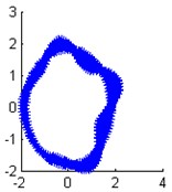
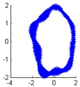
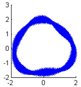
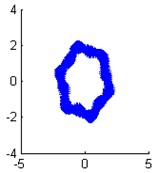
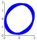
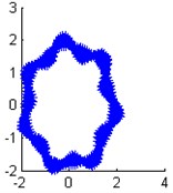
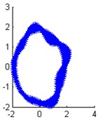
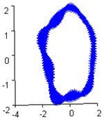
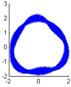
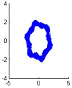
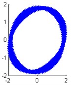
Fig. 9The identified mode shapes when the damping ratio is 0.03
a) Modal shape of the 1th order
b) Modal shape of the 2th order
c) Modal shape of the 3th order
d) Modal shape of the 4th order
e) Modal shape of the 5th order
f) Modal shape of the 6th order
Fig. 10The identified mode frequencies when the damping ratio is 0.03 with 5 % measurement noise
a) FFT of the 1th order
b) FFT of the 2th order
c) FFT of the 3th order
d) FFT of the 4th order
e) FFT of the 5th order
f) FFT of the 6th order
Table 6MAC of modal shapes when the damping ratio is 0.03 and with 5 % measurement noise
FEA method | SIPCE+ Direct matrix assemble | SIPCE+ Least-square matrix substitution | PCA+ Least-square matrix substitution | |||
Order of modal shape | Order of identified modal shape | Order of identified modal shape | Order of identified modal shape | |||
1 | 2 | 0.6554 | 2 | 0.8784 | 2 | 0.6477 |
2 | 1 | 0.6180 | 1 | 0.6842 | 1 | 0.6201 |
3 | 3 | 0.7833 | 3 | 0.5639 | 3 | 0.7594 |
4 | 4 | 0.5284 | 4 | 0.4274 | 4 | 0.5225 |
5 | 6 | 0.7280 | 6 | 0.6277 | 6 | 0.7163 |
7 | 5 | 0.9038 | 5 | 0.6563 | 5 | 0.9039 |
Table 7 is the comparison of time cost and memory cost between the two methods.
Fig. 11The identified mode shapes when the damping ratio is 0.03 with 5 % measurement noise
a) Modal shape of the 1th order
b) Modal shape of the 2th order
c) Modal shape of the 3th order
d) Modal shape of the 4th order
e) Modal shape of the 5th order
f) Modal shape of the 6th order
Table 7The comparison of time and memory consumption
Methods | Time cost (s) | Memory cost (MB) |
SIPCE+ Direct matrix assemble | 109.216 | 1008.1 |
SIPCE+ Least-square inverse matrix | 97.343 | 213.7 |
PCA+ Direct matrix assemble | 344.940 | 4367.5 |
PCA+ Least-square inverse matrix | 147.325 | 1415.8 |
4.4. Results analysis
1) Fig. 5-8 and Table 3-6 show the new method (SIPCE with direct matrix assemble) identifies the three-dimensional structures well, and it’s robust to interference noise, the 5 % Gauss measure noise has little affected to the identified accuracy.
2) For three-dimensional modal shapes, Table 3-6 show the new method (SIPCE+ Direct matrix assemble) has higher identified accuracy in four modes (3-7 modes), it’s more accuracy than the previous method (PCA+ Least-square matrix substitution) in general. And Table 6 emphasizes the method of direct matrix assemble is the crux of the high accuracy.
3) Table 7 shows this SIPCE sharply reduces the time and memory consumption. When the response signal matrix is assembled, the size of assembled signal matrix is much larger than before. So, this paper uses SIPCE to solve the PCA model of directly matrix assembly. The SIPCE’s advantage of low space-time complexity is obvious.
4) The 6th order modal parameters are missing because of its small modal contribution in structure’s dynamic response measurements.
5) In the simulation verification of cylindrical shell with two simple supported ends, there are two modal shapes with phase difference corresponding to one order natural frequency. Three-dimensional structure is more complex than one-dimensional structure, so there is always large error for identified three-dimensional modal shapes.
The authors declare that there is no conflict of interest regarding the publication of this article and regarding the funding that they have received.
5. Conclusions
This paper proposes a SIPCE algorithm and a new modal shape matrix assemble method for OMA of three-dimensional structure. The new method identifies three-dimensional modal parameters more accurately than the previous way. What’s more, the new method has lower time and space complexity, so it’s much more suitable to be embedded into hardware equipment. However, this method just applied to time invariant three-dimensional structure. The OMA based on adaptive method for time varying three-dimensional structure is the future research direction.
References
-
Reynders E. System identification methods for (operational) modal analysis: review and comparison. Archives of Computational Methods in Engineering, Vol. 19, Issue 1, 2012, p. 51-124.
-
Wang B. T., Cheng D. K. Modal analysis of mDOF system by using free vibration response data only. Journal of Sound and Vibration, Vol. 311, Issue 3, 2008, p. 737-755.
-
Han S., Feeny B. Application of proper orthogonal decomposition to structural vibration analysis. Mechanical Structures and Signal Processing, Vol. 17, Issue 5, 2003, p. 989-1001.
-
Wang B. T., Cheng D. K. Modal analysis of mdof structure by using free vibration response data only. Journal of Sound and Vibration, Vol. 311, Issue 3, 2008, p. 737-755.
-
Poncelet F., Kerschen G., Golinval G. C., et al. Output-only modal analysis using blind source separation techniques. Mechanical Systems and Signal Processing, Vol. 21, Issue 6, 2007, p. 2335-2358.
-
Zhou Wenliang, Chelidze D. Blind source separation based on vibration mode identification, Mechanical Systems and Signal Processing, Vol. 21, Issue 8, 2007, p. 3072-3087.
-
Kerschen G., Poncelet F., Golinval J.-C. Physical interpretation of independent component analysis in structural dynamics. Mechanical Systems and Signal Processing, Vol. 21, 2007, p. 1561-1575.
-
Bai Junqing, Yang Guirong, Wang Cheng Modal identification method following locally linear embedding. Journal of Xi’an Jiaotong University, Vol. 47, Issues 1-85, 2013, p. 89-100.
-
Peason K. On lines and planes of closest fit to systems of point in space. Philosophical Magazine, Vol. 1901, Issue 2, 11, p. 559-572.
-
Kerschen G., Golinval J., Vakakis A. F., et al. The method of proper orthogonal decomposition for dynamical characterization and order reduction of mechanical systems: an overview. Nonlinear dynamics, Vol. 41, Issue 1, 2005, p. 147-169.
-
Cheng W., Jin G., Junqing B. Modal parameter identification with principal component analysis. Journal of Xi’an Jiaotong University, Vol. 47, Issue 11, 2013, p. 97-105.
-
Hansen P. C. Truncated singular value decomposition solutions to discrete ill-posed problems with ill-determined numerical rank. SIAM Journal on Scientific and Statistical Computing, Vol. 11, Issue 3, 1990, p. 503-518.
-
Wang C., Guan W., Gou J., et al. Principal component analysis based three-dimensional operational modal analysis. International Journal of Applied Electromagnetics and Mechanics, Vol. 45, Issues 1-4, 2014, p. 137-144.
-
Wang J., Wang C., Zhang Y. Operational modal analysis of three-dimensional structures by second-order blind identification and least square generalized inverse. Journal of Vibroengineering, Vol. 19, Issue 4, 2017, p. 2857-2872.
-
John A. L., Michel V. Nolinear Dimensionality Reduction. Springer, 2007, p. 22-37.
-
Yang J. N., Lei Y., Lin S., et al. Identification of natural frequencies and dampings of in situ tall building using ambient wind vibration data. Journal of Engineering Mechanics, Vol. 130, Issue 5, 2004, p. 570-577.
-
Wold H. O. A. Nonlinear Estimation by Iterative Least Square Procedures. Wiley, London, New York, 1968.
-
Wold S. Pattern recognition by means of disjoint principal components models. Pattern Recognition, Vol. 8, Issue 3, 1976, p. 127-139.
-
Wilkinson J. H. Error analysis of direct methods of matrix inversion. Journal of the ACM (JACM), Vol. 8, Issue 3, 1961, p. 281-330.
-
Basov K. A. ANSYS and LMS Virtual Lab. Geometric Modeling. DMK Press, Moscow, 2006, p. 240.
-
Zhou S. D., Heylen W., Sas P., et al. Parametric modal identification of time-varying structures and the validation approach of modal parameters. Mechanical Systems and Signal Processing, Vol. 47, Issue 1, 2014, p. 94-119.
About this article

This work was financially supported by National Natural Science Foundation of China (Grant No. 51305142), the General Financial Grant from the China Postdoctoral Science Foundation (Grant No. 2014M552429), Postgraduate Scientific Research Innovation Ability Training Plan Funding Projects of Huaqiao University (Grant No. 1511314011).
