Abstract
With the increased running speed of trains, the aerodynamic noise of trains becomes increasingly obvious. Reducing aerodynamic noises has become one of keys to controlling the noise of high-speed trains. This paper conducted a numerical simulation on the aerodynamic noise of head of the high-speed train. Firstly, this paper established a mathematical-physical model for the three-dimensional turbulent flow field of a high-speed train, adopted standard - equation turbulent model and broadband noise source model to compute the aerodynamic noise sources of the high-speed train and applied three-dimensional transient large eddy simulation (LES) to compute the external unsteady flow field of the high-speed train after obtaining noise sources. Based on the unsteady flow field, then this paper applied FW-H equations to compute the far-field aerodynamic noise of the high-speed train. After obtaining the unsteady fluctuation pressure on the surface of the train, this paper computed the radiation characteristics of aerodynamic noises around the high-speed train based on the boundary element method (BEM). Researched results showed: The main aerodynamic noise sources of the high-speed train were at the nose tip of head train; fluid separation and recombination were main reasons for the aerodynamic noise of the high-speed train; vortexes in the position of head train were striped and horseshoe-shaped or hairpin vortexes were mainly in the area of tail train; in addition, vortexes were symmetrically distributed along the longitudinal symmetry plane of train; dipole noises were mainly distributed in the area of head train, whose main energy was decreased with the increased frequency; the quadrupole noise of aerodynamic noises of the high-speed train was mainly distributed in the wake flow area of tail train; when the high-speed train ran at the speed of 300 km/h, the maximum sound pressure level of far-field observation points was 76.8 dB; additionally, aerodynamic noises in the far field were mainly a broadband noise, whose main energy was within the frequency range of 1250 Hz to 3150 Hz. Finally, the improved NSGA-II algorithm was used to conduct a multi-objective optimization for the head shape. The aerodynamic drag of the high-speed train could be most reduced by 6.74 %, and the dipole aerodynamic noise source could be most reduced by 8.34 dB. The improved NSGA-II algorithm has an obvious effect on the multi-objective optimization of the head shape.
1. Introduction
With the constant increase of running speed of trains, many problems which are neglected at low speeds have become increasingly obvious and had an influence on the development of trains to a large extent [1-5]. Problems in the aspect of aerodynamics are particularly prominent, like air drag and aerodynamic noise. When a train runs at a low speed, air drag takes up a very small proportion compared with other drags. When the speed of the train is increased to 200 km/h and 300 km/h respectively, the proportion of air drag will increase to about 70 % and 80 % respectively [6-8]. Due to the increased train speed, air fluctuation pressure waves acting on the surface of train body increase rapidly; the running stability of the train will be seriously affected; aerodynamic noise will be increasingly obvious. Researches show that aerodynamic noises will exceed wheel-rail noises and become the main noise source of a running train when the train runs at the speed of more than 300 km/h [9, 10]. The size of aerodynamic noises is mainly affected by the speed when a high-speed train runs and approximately in direct proportion to 6 to 8 [7, 8]. With the constant increase of running speed, aerodynamic noises will dramatically increase. The increase of railway noises will have a serious impact on the environmental comfort in the train and the life of residents along railway and thus affect the development of high-speed trains. The aerodynamic noise of high-speed trains has a huge influence on the construction and development of railways. Reducing aerodynamic noise has become one of problems urgently needing to be addressed in order to develop high-speed trains [11].
With the constant development of computing technology and the perfection of fluid mechanics theory, researchers have started to adopt the numerical simulation method to study the sound production problem of fluid. In this case, computational aero-acoustics have been proposed at the right moment and become a powerful method of studying aero-acoustics [12]. T. Sassa combined BEM with finite element method to simulate the noise on the surface of the high-speed train and analyze noise characteristics [13]. Then, Takehisa adopted LES and Green function to simulate the distribution of dipole sources on the surface of the high-speed train and formed some knowledge of the distribution rule of dipole on the surface of the train [14, 15]. Li used BEM to simulate and analyze interior sound field. Analyzed results were consistent with experimental data in the low frequency band, but there were large errors in the mid-high frequency bands [16]. Liu preliminarily concluded and summarized the computational methods of aerodynamic noises of the high-speed train [17]. Lu theoretically studied and numerically probed into the distribution of fluctuation pressure on the surface of trains [18, 19]. Wang combined LES with FW-H equations to predict exterior noises [20]. Tian predicted and analyzed the interior aerodynamic noise of cabin of the high-speed train [21]. Yang applied Fluent to simulate and analyze the external flow field and aerodynamic noise of current collection parts of the high-speed train with and without an air deflector [22]. Based on delayed detached eddy simulation (DDES) and FW-H equations, Zhu predicted the flow field characteristics and dipole distribution rule of a simplified bogie only containing wheel-sets and framework with the scaling of 1:10 and verified the correctness of numerical simulation through wind tunnel test. Results showed that the aerodynamic noise of bogies was a broadband noise and the bogie had main single-frequency noise. The first-order frequency of the bogie was mainly caused by the vortex shedding of axle; the second basic frequency was mainly caused by the interaction between axle and wheel; in addition, the first-order frequency was related to the lift of bogies and the second-order frequency was related to the drag of bogies [23]. Lee verified and obtained the shape of low-noise pantograph head and the noise reduction effect of new-type pantograph through optimizing the structural shape of pantograph head, adopting new-type and low-noise PS207 pantograph and conducting wind tunnel test [25, 26]. Liu established a mathematical model for the three-dimensional turbulent flow field of head of the high-speed train, used Lighthill acoustic analogy theory to compute the far-field aerodynamic noise of the high-speed train and applied a broadband noise model to compute aerodynamic noise sources on the surface of the high-speed train head [27]. Due to the limitation of conditions, the aerodynamic noise of high-speed railway was mainly studied from the aspect of theoretical research and experiments. Incompressible fluid model was used for handling the numerical simulation. In addition, the sound pressure on the surface of train and sound pressure of field points were mostly simulated and computed, but the description of distribution and propagation situation of aerodynamic noises in space was not clear.
Based on the above researches, this paper mainly involved the flow field characteristics of the high-speed train, analysis of aerodynamic noises and research on the sound radiation of aerodynamic noises based on acoustic BEM. In addition, this paper combined standard - equation turbulent model with a broadband noise source model to study the distribution and intensity of aerodynamic noise sources of the high-speed train. Meanwhile, this paper combined LES with Lighthill acoustic analogy theory to analyze the far-field aerodynamic noise of the high-speed train and applied acoustic BEM to study the sound radiation of aerodynamic noises of the high-speed train after obtaining the fluctuation pressure field on the surface of the high-speed train.
2. Mathematical model
2.1. LES method
The foundation of LES is the algorithm of vortex design of turbulent flow. Vortex theory holds the opinion that turbulent flow is composed of many vortexes of different sizes. Large-scale vortexes have an obvious influence on the primary motion of fluid. Small-scale vortexes have impacts on the flow of large-scale vortexes through nonlinear function. Such vortexes of different scales presented constant changes and produced pressure fluctuation of different scales and frequencies under their interaction with turbulent flow [28-30]. Dipole sources in the basic equation of aero-acoustics (FW-H equation) were just determined by fluctuation pressure of such flow field boundary.
The basic thought of LES is to filter the vortexes of flow field of turbulent transient motion through LES filter. After vortexes less than a certain scale in the flow field are filtered out, the motion of remaining large-scale vortexes is solved through directly applying N-S equation. Filtered small-scale vortexes compute their motion through additional equation. According to the basic thought of LES, a method had to be adopted to distinguish large-scale vortexes to be solved and modeled small-large vortexes. Different from RANS, LES adopted spatial average method to decompose the variable into and sub-grid variable in -. could adopt the equation raised by Leonard as follows:
wherein, was filter function. Common filter functions are Gaussian function and cap-type function. Widely-used cap-type function with simple form was obtained:
wherein, referred to average grid size; three dimensions , , and stood for grid sizes in the direction of , and . When , LES was transformed into DNS [31, 32].
2.2. FW-H equations
Acoustic analogy theory was initially proposed by Lighthill. After it was promoted by Curle, Ffowcs-Williams and Hawkings, Ffowcs Williams-Hawking equation [33] (FW-H equations for short) was obtained. Its differential form was:
wherein, referred to air pressure; stood for normal direction; represented sound velocity; was normal velocity; meant static pressure; was Lighthill pressure tensor; was function; was Heaviside function.
3. Numerical model
As LES technology has very high requirements for grids, large computer memory and long computation time have to be occupied. Under current technical conditions, it is very difficult to realize the numerical computation of LES of three-dimensional turbulent flow of the high-speed train including multiple trains. Reference [21] pointed out that head of the high-speed train was a main aerodynamic noise source. Therefore, this paper focused on studying the aerodynamic noise problem of train head. In addition, strong vortex shedding would appear in the rear section of train head if only train head was selected as a computational model to simulate the flow field. On the one hand, such vortex shedding was not consistent with the actual situation; on the other hand, it had great influence on the flow field around the rear section of train head. As a result, the computational model of this paper was composed of train head and tail which had the same shape so that the flow field in the rear section of train head was closer to the actual situation.
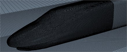
The geometric size of the high-speed train head was used to establish a computational model. To reduce computational model and difficulty, parts including the bogie, wheel rail and pantograph of train body were simplified in the process of modeling. Suppose the surface of train body was smooth and the train window on the surface of train body and gap in the connection of train doors were neglected. The model with the scaling of 1:8 was adopted to compute the aerodynamic noise of the high-speed train. The simplified model of the high-speed train was shown in Fig. 1.
Fig. 1Geometric model of the high-speed train
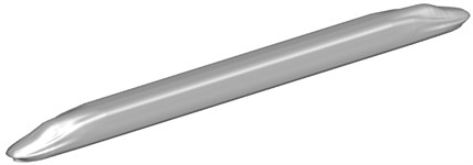
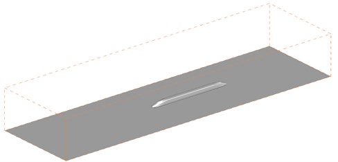
Fig. 2 displayed the computational domain for the aerodynamic noise of the high-speed train. Train length was taken as the benchmark. Therefore, the length of its computational domain was 4 long, wide and 0.5 high. The nose tip of head train was away from the inlet. The nose tip of tail train was 2 away from the outlet. The train was 0.2 m away from the ground where the track was. The inlet boundary of high-speed train was set as velocity inlet condition and velocity was 300 km/h in the case of computation. The outlet boundary of tail train of the high-speed train was set as pressure outlet condition. The ground was set as slip ground, whose slip velocity was the running speed of train. Other outer boundaries of high-speed train were set as symmetrical boundary conditions.
Fig. 2Computational domain for aerodynamic noises
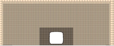
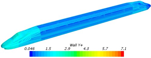
Trimmer grid was adopted to divide the grids of computational domain of the high-speed train. Grids of the boundary layer were divided on the surface of the high-speed train. In the meanwhile, the area of grid encryption was set around the high-speed train. The maximum grid size on the surface of train was 10 mm; the maximum size of space grids was 150 mm; the maximum size of volume grids in the encryption area surrounding the train was 20 mm. To eliminate the impact of train surface on fluid flow, the boundary layer was divided on its surface. The first boundary layer was 0.01 mm thick, whose growth rate was 1.2. The grids of the boundary layer had an overall thickness of 8 layers. The space grids of high-speed train were shown in Fig. 3. Fig. 4 displayed the contour for the distribution of + on the surface of the high-speed train. As displayed form the figure, most of + values on the surface were less than 1 when LES method was applied to compute the aerodynamic noise of high-speed train. Therefore, the computational grids of this paper satisfied the demand of grids for independence [8]. The sliding grid technology was used to simulate the motion of the high-speed train.
Fig. 3Schematic diagram for the grids of the high-speed train
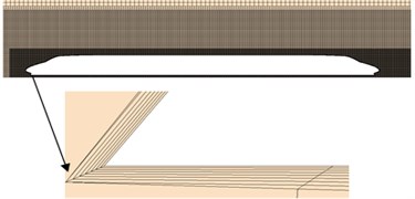
a) The whole train
b) Cross-section
c) Head train
Fig. 4Contour for Y+ of the high-speed train
4. Flow field characteristics around the train head
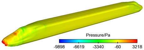
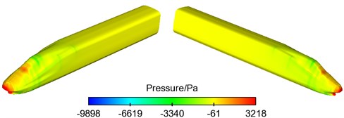
When the high-speed train ran under the working condition of a steady speed, airflow velocity decreased as air flow was hindered at the nose tip of windward side of train head and in the front of air deflector. A main area of positive pressure was formed. The maximum pressure was around 3218 Pa at the nose tip of head train and in the position of tail train. A part of air flew along the surface of train body. When air flew to the tail end of train nose and around the front windshield, an area of negative pressure was formed due to the sudden change of curvature of train surface and the separation of airflow near the wall and on the surface of train. A part of airflow near the wall was mixed at the bottom of train body and separated from train body when reaching the middle part of head train, forming an area of negative pressure. Another part of airflow was directly crushed by train nose and air deflector into the bottom of train and separated from the surface of train body, forming a large area of negative pressure. The maximum negative pressure amounted to –9898 Pa. In the rear of head train and the position of tail train, the pressure of train body was within the range of ±300 Pa as fluid on the surface of train body was relatively stable compared with that in the position of head train, which was consistent with the situation in the actual operation of train and indicated the rationality of simplification and analysis of flow field model. Fig. 5 displayed the contour for the pressure distribution on the surface of train when the train ran under the working condition of 300 km/h. Pressure distribution around train body was shown in Fig. 6. Thus, it was clear that the maximum pressure of the whole train was at the nose tip of head train which was the position of stagnation points for the pressure of nose tip.
Fig. 5Contour for the pressure on the surface of the high-speed train
a) The whole train
b) Head train
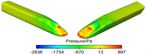
c) Tail train
Fig. 6Contour for pressure around the high-speed train
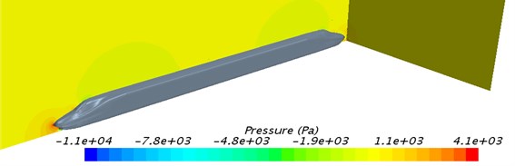
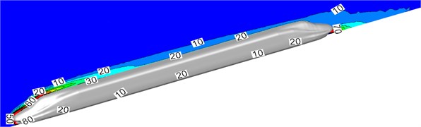
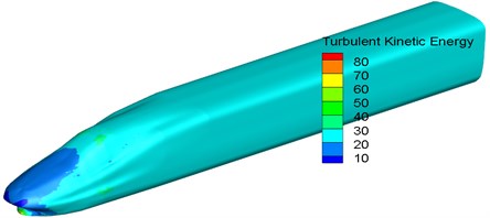
Fig. 7 displayed the distribution of surface turbulent kinetic energy in the area of the whole train and the longitudinal central plane of train body. As displayed from Fig. 7, higher turbulent kinetic energy was at the nose tip of head train and in the rear of nose tip of tail train. In addition, fluid separation and recombination alternated in this area. Therefore, it could be seen that the nose tip of head train was the main aerodynamic noise source of the high-speed train, followed by the window of head train.
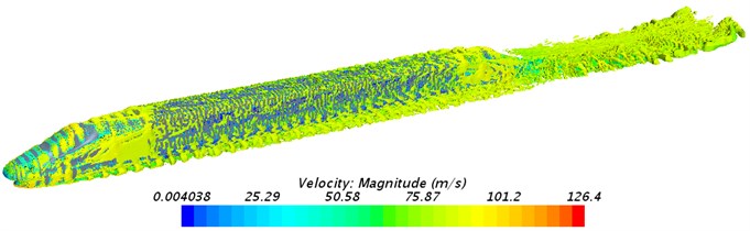
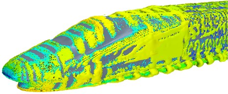
Fig. 8 displayed the contour for the distribution of vorticity based on Q-criterion (scale was 1000/s2) when the high-speed train ran at the speed of 300 km/h. As displayed from Fig. 8, the streamlined position of train head had a great impact on air flow. Firstly, airflow had a high speed when reaching the nose tip of head train and the position of tail train. As the nose tip of head train blocked airflow, airflow separated at the nose tip of head train, but airflow did not vertically flow to the surface of train along the normal direction on the surface of nose tip. According to the actual situation, the incidence direction of airflow formed a certain angle with the surface of train body. Such flow phenomenon caused by the incidence of airflow forming a certain angle with solid surface was similar to turbulent flow model formed by the oblique incidence of airflow to plate. A layer of fluid close to solid surface had a low flow velocity due to the viscosity of solid surface. Fluid away from solid surface had a high flow velocity. Then, the flow velocity of fluid increased with the increase of its distance from solid surface and flow velocity showed the phenomenon of stratification.
Fig. 7Contour for the distribution of turbulent kinetic energy of train head
a) The whole train
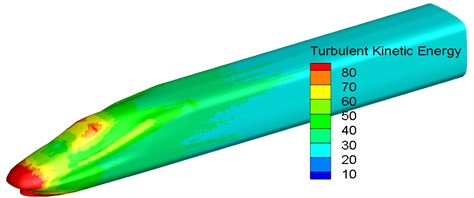
b) Head train
c) Tail train
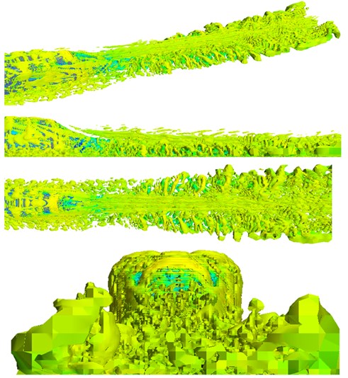
On the other hand, fluid itself owned viscosity. Fluids with a high flow velocity and a low flow velocity would interact under the action of viscous stress inside fluids, which made a layer of thin fluid close to solid surface present the trend of gradually getting close to solid surface in the process of flowing forward on the whole. Under high velocities, such a trend of getting close to the wall would finally develop into local backflow and further show a series of low-velocity stripes in the position close to solid surface, as shown in Fig. 8(a). Low-velocity stripes were the initial stage of vortex development. Low-velocity stripes grew continuously and the viscosity of solid surface weakened the constraint of them. At this time, low-velocity stripes would show oscillation. Then, vortexes rolled, shed, stretched forward along the flow direction and formed horseshoe-shaped or hairpin vortexes. As a whole, horseshoe-shaped or hairpin vortexes were the most common turbulent vortexes caused by high-speed train. On the other hand, turbulent vortexes shedding from tail train had a large scale, whose main energy was contained in these large-scale vortexes with relatively intensive vorticity. Along the flow direction, vortexes stretched and broke into smaller-scale ones. The range of vortex distribution was expanded, as shown in Fig. 8(c). In the area of wake flow, turbulent flow was symmetrically distributed along the longitudinal symmetry plane of train. In addition, fluid separated at the window of tail train. Separated airflow was striped vortex. Vortexes at the bottom of nose tip of tail train had great intensity, most of which were horseshoe-shaped or hairpin vortexes in the aspect of distribution shape. Thus, it could be seen that fluid separation and recombination were main reasons for the formation of the aerodynamic noise of the high-speed train.
Fig. 8Contour for the distribution of vorticity of the high-speed train
a) The whole train
b) Head train
c) Tail train
5. Aerodynamic noises of head of the high-speed train
5.1. Aerodynamic noise sources
Fig. 9 displayed the contour for the distribution of dipole noise on the surface of the high-speed train. As displayed from Fig. 9, the streamlined train head of the train had a large sound power level, especially the top of streamlined head. Streamlined train tail had a small sound power level. Thus, it was clear that the main sound sources of the train were where airflow was separable easily and turbulent motion was drastic. Therefore, optimizing the shape of train head and body and reducing the disturbance of concavo-convex objects on airflow were the effective method of reducing aerodynamic noises. In addition, it could be seen from Fig. 9 that the sound power level of train body decreased along train axle when it kept a certain distance from the streamlined part of train head. This rule showed that the simplified model in this paper reasonably shortened train model and did not change the basic rule of aerodynamic noise distribution of train body.
Fig. 9Distribution of dipole noise of the high-speed train
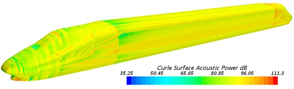
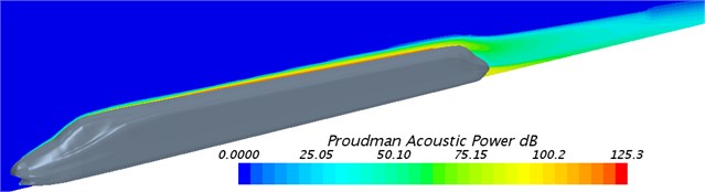
Fig. 10 displayed the contour for the distribution of quadrupole noise of flow field around the high-speed train. As displayed from Fig. 10, the noise around the high-speed train was mainly in the rear of tail train; wake flow had an obvious impact on the quadrupole noise of the high-speed train; quadrupole noise gradually increased, whose distribution range became wider and wider. In the vertical plane, the distribution of quadrupole noise was smaller when it was further away from the ground.
Fig. 10Distribution of quadrupole noise of the high-speed train
a) Longitudinal direction

b) Vertical direction (0.1 m away from the ground

c) Vertical direction (0.2 m away from the ground

d) Vertical direction (0.3 m away from the ground
Fig. 11 displayed the relationship between the maximum sound power level and the running speed of train in different positions of the high-speed train. As displayed from Fig. 11, the maximum sound power level in different positions of train body obviously increased with the increased running speed of train. Reference [5] pointed out that the relationship between the maximum sound power level and the running speed of train could be explained as:
wherein, 200 km/h. Polynomial fitting was used to determine unknown parameters and obtain the corresponding function relationship between the maximum sound power level and the running speed of train shown in Fig. 11. The maximum sound power level at the nose tip of head train and running speed satisfied the following function relationship:
The function relationship between the maximum sound power level at the nose tip of tail train and the running speed of the high-speed train was:
Fig. 11Distribution of sound power levels at the nose tip of train
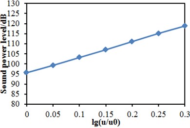
a) Nose tip of head train
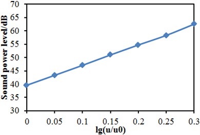
b) Nose tip of tail train
5.2. Distribution characteristics of aerodynamic noises in the far field
Fig. 12 displayed the arrangement diagram of observation points for the far-field aerodynamic noise of the high-speed train. 65 observation points of noises were arranged in the places which were 7.5 m away from the center line of track and 0.35 m high from the track surface and along the longitudinal direction. The distance between two adjacent observation points of noise was 0.1 m. These observation points of noises were named as z1, z2, …, z65.
Fig. 12Arrangement of observation points of far-field aerodynamic noise
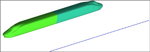
Fig. 13 displayed the distribution curves of far-field sound pressure levels along the longitudinal direction of the train when the high-speed train ran at the speed of 300 km/h. The arrangement of observation points was shown in Fig. 12. As displayed from Fig. 13, the sound pressure level of aerodynamic noises of the high-speed train gradually decreased along the flow direction of airflow; the sound pressure level of far-field aerodynamic noises reached a local maximum where there was a transition from the streamlined position of head train to the non-streamlined position of head train and from the non-streamlined position of tail train to the streamlined position of tail train. At the observation point z13, the maximum sound pressure level was 76.8 dB. The sound pressure level of head train was decreased by 3.2 dB most while the sound pressure level of tail train was decreased by 2.9 dB most.
Fig. 13Distribution of sound pressure levels of far-field aerodynamic noises (300 km/h)
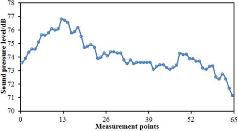
Fig. 14 displayed the distribution curves of far-field sound pressure levels along the longitudinal direction of the train when the high-speed train ran at the speed of 350 km/h. The arrangement of observation points was shown in Fig. 12. Through comparing Fig. 12 with Fig. 13, it could be seen that the far-field aerodynamic noise of the high-speed train increased with the increased running speed of train and the maximum sound pressure was increased by 3.3 dB. The distribution curves of sound pressure levels of aerodynamic noises showed approximately the same change rule: The sound pressure levels of aerodynamic noises were gradually decreased along the flow direction of airflow; the sound pressure level of far-field aerodynamic noise reached a local maximum where there was a transition from the streamlined position of head train to the non-streamlined position of head train and from the non-streamlined position of tail train to the streamlined position of tail train; at the observation point z13, the maximum sound pressure was 80.1 dB.
Fig. 14Distribution of sound pressure levels of aerodynamic noise of the high-speed train (350 km/h)
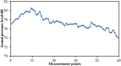
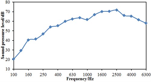
Fig. 15 displayed the distribution diagram for 1/3 octave of observation point z13 when the high-speed train ran at the speed of 300 km/h. As displayed from Fig. 15, the far-field aerodynamic noise of the high-speed train was a kind of broadband noise and existed in a wide range of frequencies, whose main energy was within the frequency range of 1250 Hz to 3150 Hz. Sound pressure level was 71.2 dB when center frequency was 2500 Hz.
Fig. 15Analysis on 1/3 octave of observation point z13
5.3. Distribution characteristics of aerodynamic noises in the near field
The acoustic BEM was used to identify the aerodynamic noise sources of bogies and the propagation characteristics of aerodynamic noises. In the flow field, the time-domain signals of fluctuation pressure on the surface of the high-speed train were extracted. Meanwhile, BEM was applied to solve sound pressure on the node of sound field of receiving points. Acoustic software Virtual.Lab was used to compute the sound propagation on the surface of bogies. In addition, this paper applied sound pressure boundary conditions to map the fluctuation pressure obtained by CFD on the surface of the high-speed train to acoustic meshes on the surface of the high-speed train, adopted discrete Fourier transform to complete the data transfer of surface fluctuation pressure, conducted acoustic response computation and obtained the aerodynamic noise sources and aerodynamic noise radiation of the high-speed train through analyzing acoustic response. Fig. 16 displayed the acoustic meshes of the high-speed train. There were 30762 elements and 38927 nodes in total. The maximum acoustic mesh size on the surface of the high-speed train should satisfy the demand for the maximum frequency. See Eq. (7):
wherein, was the maximum acoustic mesh size; referred to the maximum computed frequency, 5000 Hz; stood for the propagation velocity of sound in the air, 340 m/s.
From Eq. (7), the maximum size 11 mm of acoustic meshes on the surface of the high-speed train could be obtained through computation. In the computation of sound propagation of aerodynamic noise in this paper, the maximum mesh size was set as 10 mm. It could be seen that the acoustic meshes computed in this paper satisfied the demand of sound propagation for the minimum wavelength.
Fig. 16Acoustic meshes of the high-speed train
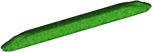
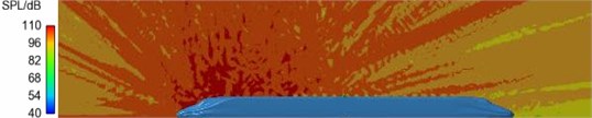
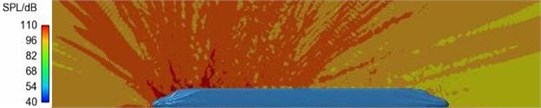
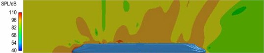
Fig. 17 displayed the contours for the distribution of sound pressure levels of dipole sources on the surface of train body at the frequency of 1000 Hz, 2500 Hz and 5000 Hz when the high-speed train ran at the speed of 300 km/h. As displayed from Fig. 17, large sound pressure levels of dipole sources were in the position of head train; main noise sources were around the bogie of head train; the maximum pressure level was 109 dB. As airflow attached on the surface of train body separated, high-intensity vortexes were formed in the area of transition from the nose tip of train head to train head, around the air deflector below the nose tip and the front windshield and in the middle of train body. Due to strong pressure fluctuation, strong dipole sources were produced, whose sound pressure level was between 90 dB and 102 dB. At the same train speed, the distribution rule of dipole sources on the surface of train body at the frequency of 2000 Hz and 5000 Hz was basically the same with that at the frequency of 1000 Hz. However, the maximum sound pressure level was decreased to some degree with the increased frequency. In addition, the distribution range of main dipole noise sources was reduced and the coverage area of main dipole noise sources became increasingly obvious, which showed that the intensity of dipole sources was gradually decreased with the increased frequency.
In addition, it could be found from the comparison of contour for the sound pressure levels of dipole sources on the surface of train body and contour for the distribution of turbulent kinetic energy on the surface of train body that dipole sources also had great intensity where the intensity of turbulent kinetic energy was great. It was because the generation of turbulent kinetic energy and dipole sources was related to the complex situation of flow field. The more complex the flow field on the surface of train body was, the greater the intensity of turbulent flow would be, the greater turbulent kinetic energy on the surface of train body would be and the greater the intensity of dipole sources would be. Therefore, reducing the intensity of turbulent flow on the surface of train body could reduce the generation of aerodynamic noise when train ran. Besides, the distribution rule of dipole sources could be predicted through observing the distribution situation on the surface of train body in the flow field.
Fig. 17Distribution of sound pressure levels of sound sources of the high-speed train
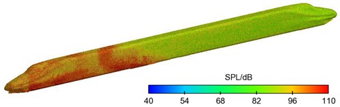
a) 1000 Hz
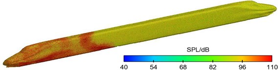
b) 2500 Hz
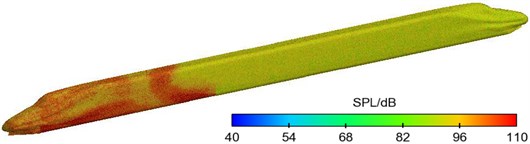
c) 5000 Hz
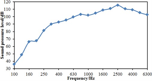
This paper conducted numerical simulation for dipole sources on the surface of train, used BEM to conduct simulation analysis on the radiation sound field of dipole sources on this basis, studied the radiation characteristics of aerodynamic noises of the high-speed train and laid a foundation for controlling aerodynamic noises along railway routes. When the high-speed train ran at the speed of 300 km/h, dipole sources were taken as boundary conditions. Suppose the ground totally reflected noise, indirect BEM was applied to simulate and compute the distribution of sound pressure levels of radiation sound field along the longitudinal symmetry plane of high-speed train at the frequency of 1000 Hz, 2500 Hz and 5000 Hz, as shown in Fig. 18. From the analysis of Fig. 18, it could be seen that the radiation of aerodynamic noises on the longitudinal symmetry plane of the high-speed train was mainly in the position of head train. The radiation of aerodynamic noises was particularly obvious in the position of transition from the nose tip of head train to the train body of head train (above the cab of head train), which was consistent with the distribution rule of dipole sources. At the same frequency, the radiation of dipole sources of train surface on the longitudinal symmetry plane was mainly within the range of included angle from 25° to 160° formed with the ground. The intensity of radiation in the direction of track was relatively weak. In addition, the maximum sound pressure level of radiation sound field decreased from 115 dB to 96 dB and showed a decreasing tendency when the frequency increased from 1000 Hz to 5000 Hz. Additionally, the noise distribution on the sound pressure was so uniform in Fig. 18(a) and (b) because the sound wave length in the mid-high frequency will be short, and it can pass through the high speed train easily. Sound pressure levels under one-third octave at the head train nose tip of the high-speed train were extracted, as shown in Fig. 19. It is shown in Fig. 19 that the near-field sound pressure had an obvious peak value at 2500 Hz, which is consistent with the frequency of far-field peak value in Fig. 15.
Fig. 18Distribution of sound radiation of aerodynamic noises of the high-speed train
a) 1000 Hz
b) 2500 Hz
c) 5000 Hz
Fig. 19Sound pressure levels under one-third octave at head train nose tip
5.4. Experimental verification of the computational model
The mentioned model used for computing near-field and far-field aerodynamic noises of the high-speed train was very complicated, so its correctness should be verified by its experimental test. The experimental test was conducted in a wind tunnel experimental section with 8 m×6 m. The wind tunnel was a closed in-series high-speed wind tunnel. As for the experimental section, the cross-section area was 8 m×6 m; length was 15 m; stable wind speed ranged within 20 m/s-70 m/s. In order to reduce impacts of floor boundary layers, a dedicated floor device for train experiments was installed in the experimental section. Front and rear edges of the floor were processed into a streamline type, so interference to airflows could be reduced. The mode used in the experiment was a 2-train formation model including a head train and a tail train. The train model was a metal frame structure, wherein the exterior was shaped by wood. The model scale was 1:8. The experimental model was shown in Fig. 20(a). Head and tail shapes of the train model were completely symmetrical. Based on position characteristics of several major noise sources of the train model, the experiment expected to obtain characteristics and distribution of corresponding noises. Free field microphones [34] were arranged outside flow fields of the experimental section, so radiated noises of aerodynamic noise sources of the model were tested, and radiation characteristics of the train noise sources could be known, as shown in Fig. 20(b). It is shown in the figure that microphones were arranged on the surface and in the far field of the high-speed train, where they were used to test near-field and far-field radiation noises respectively. The radiation noise was compared with numerical simulation results, so correctness of the numerical model could be verified, as shown in Fig. 21. It is shown in Fig. 21 that the experimental results and numerical simulation results differed a lot in the low frequency. The boundary conditions in the low frequency had obvious impacts on computational results, so boundary conditions of the numerical simulation could hardly be simulated. In addition, within the analyzed frequency, experimental values were more than numerical results because numerical simulation was an ideal state and only considered radiation noises caused by the train motion, and the experimental test also contained noises caused by experimental equipment. Nevertheless, as a whole, the maximum relative error in mid-high frequency bands between numerical simulation and experimental test was lower than 5 %. Therefore, the numerical simulation is feasible and can replace experimental test to study aerodynamic noises of the high-speed train.
Fig. 20Experimental test on aerodynamic noises of the high-speed train
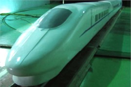
a) Experimental model
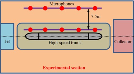
b) Arrangement of sensors
Fig. 21Experimental verification of the numerical model of the high-speed train
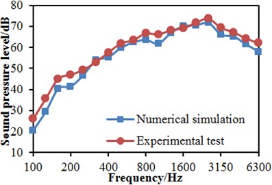
a) Near-field radiation noises
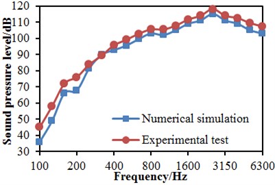
b) Far-field radiation noises
6. Multi-objective optimization of aerodynamic noises of the high-speed train
The computational results showed that the head shape of the high-speed train could seriously affect aerodynamic performance, and then seriously affect the radiation noise. During designing the head shape of the high-speed train, factors such as drag, lift, crosswind safety performance and aerodynamic noises during train running should be considered comprehensively, where conflicts could take place among the objectives. Therefore, designing the head shape of the high-speed train is a multi-objective optimization problem [35, 36]. At present, during optimization design on the head shape, many head shape schemes are listed in general; tunnel experiments and numerical computation are then used for comparative selection; finally, the design is improved according to operation conditions. In essence, the method is an optimal method which excessively depends on engineering experience, and the finally selected head shape is not always the best. In order to overcome these defects and obtain the optimal head shape, direct optimization must be adopted. When the constraint conditions are satisfied, direct optimization design adopts a mathematic method to maximize or minimize design objectives as much as possible. Therefore, the head shape design of the high-speed train could be converted into a multi-objective optimization problem. Through parameterized modeling for the head shape of the high-speed train, optimization design variables are selected; optimization objective values were obtained through computing aerodynamics of the high-speed train; values of optimization design variables could be updated automatically by the multi-objective optimization algorithm. The paper will establish a multi-objective optimization model of the streamline head shape of a high-speed train, and conduct multi-objective optimization design on drag and noise reduction to the streamline head shape of the high-speed train with aerodynamic drag and noise sources as the optimization objectives.
Based on the commercial software CATIA, the three-dimensional parameterized model of the high-speed train was established, so the streamline head shape could be deformed automatically. For this purpose, the following steps should be completed in succession: the CATSCRIPT script file of CATIA was used to conduct parameterized modeling of the left half head shape. The complete train model could be established by the streamline head shape through translation and symmetry operations. The MATLAB program was used to modify parameter values in the CATSCRIPT script file. Therefore, the streamline head shape of the high-speed train could be deformed through running the CATSCRIPT script file. The streamline head shape of the high-speed train was highly symmetric, so the solid modeling should only be conducted on the left half head shape. In the paper, several B-Spline curved faces were used to approach the outer surface of the left half head shape of the high-speed train. The B-Spline curved face was composed of a series of B-Spline curves, and the B-Spline curve was composed of a series of control points on the streamline head surface. According to the streamline head shape of the high-speed train, 160 control points were established on the streamline head surface; the 160 control points were used to establish 12 B-Splines; the 12 B-Spline curves were used to establish 7 B-Spline curved faces. Therefore, the streamline head shape of the high-speed train was established, as shown in Fig. 22. In order to conduct analysis more easily, the 12 B-Spline curves were numbered, namely C1-C12.
Fig. 22Streamline head shape of the high-speed train
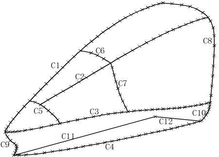
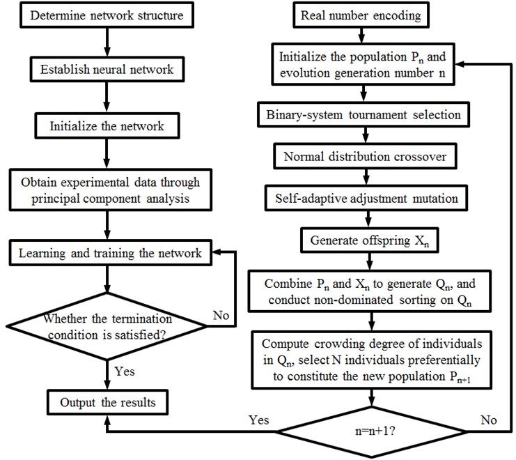
In order to optimize the streamline head shape of the high-speed train, 6 design variables were established, which were corresponding to longitudinal symmetric line C1, lateral vertical maximum profile line C2, horizontal maximum external profile line C3, train bottom horizontal profile line C4, middle auxiliary profile line C7 and nose tip altitude line C9. With increased streamline length, aerodynamic performance of the high-speed train would be improved obviously. However, blind increase of the streamline length would reduce internal space of the train. Therefore, the paper optimized the streamline head shape to improve aerodynamic performance of the high-speed train when the streamline length is constant. At present, some scholars have studied optimization of the head shape. In order to improve aerodynamic performance of a high-speed train, Zhang [37] took aerodynamic drag of the head train and aerodynamic lift of the tail train as optimization objectives and used the NSGA-II algorithm to conduct a multi-objective optimization design on the head shape. In order to improve crosswind aerodynamic performance of the high-speed train, Yu [38] took lateral force and lift of the high-speed train under crosswind as optimization objectives, and used the NSGA-II algorithm to conduct a multi-objective optimization design on the head shape. Obviously, the NSGA-II algorithm is widely used in the multi-objective optimization of the head shape. However, these applications only took the traditional NSGA-II model as an optimization algorithm. The distance crowding mechanism of the traditional NSGA-II algorithm is unstable, so the solution set distribution was not always satisfactory, and the subsequent clipping strategy was also unstable. In addition, the algorithm is deficient in high computation complexity, long computation time, lack of elitist strategy and request for manual assignment of shared variables. Therefore, the mentioned applications would be deficient inevitably because they used the NSGA-II algorithm to conduct a multi-objective optimization of the head shape. Aiming at this problem, the paper aimed to improve the NSGA-II algorithm. Improvement scheme of NSGA-II mainly focuses on two aspects: Pareto solution set distribution is strengthened; convergence speed is increased. The improved NSGA-II algorithm takes a BP neural network model as the optimization evaluation system [39-43]. During the genetic process, a normal distribution crossover operator and a self-adaptive adjustment mutation operator are adopted. Therefore, search for excellent individuals is accelerated; diversity of search space and populations is improved; and new populations have higher adaptability, namely a Pareto optimal solution set could be obtained. Flow chart of the algorithm is shown in Fig. 23. Specific process is as follows: a) An initial population with individuals is generated randomly; rapid non-dominated sorting is conducted on the population; grade values of all individuals in the population are initialized; number of evolution generations is 0. b) Individuals are selected randomly from for genetic operation, so the offspring generation is generated. c) and are combined, so is generated; the target function value is computed; rapid non-dominated sorting is conducted on . d) Through computing crowding degree and crowding distance of individuals in , individuals are selected preferentially to constitute the new generation of population . e) If and termination conditions are satisfied, the circulation will be stopped. Otherwise, the step b) will be started. g) BP neural network is used to evaluate the Pareto optimal solutions. f) A Pareto optimal solution set is obtained.
Fig. 23Flow chart of the improved NSGA-II algorithm
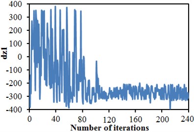
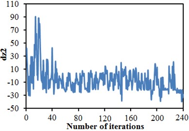
Software including MATLAB, CATIA, ICEM and FLUENT was integrated into the ISIGHT optimization software, so automatic update, automatic mesh division and automatic flow field computation of the head shape were achieved. The improved NSGA-II was used to conduct a multi-objective optimization of the head shape. 12 initial sampling points were set for 20-generation genetic computation. To complete the optimization design, the aerodynamic computation of the train with new head shape should be conducted for 240 times. Fig. 24 shows convergence curves of 6 design variables C1, C2, C3, C4, C7 and C9 with the evolution generation number. It is shown in these figures that each design variable got converged smoothly with the increased iteration number. Fig. 25 gives changing curves of optimization objectives during the optimization. Through sampling of design space with the optimization algorithm, the aerodynamic drag and dipole noise source tended to decrease as a whole. The streamline head shape of the high-speed train was gradually modified to reduced aerodynamic drag and dipole noise source.
Fig. 24Iteration curves of optimized design variables
a) Variable C1
b) Variable C2
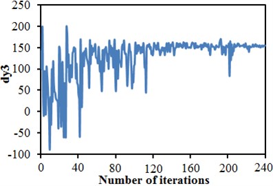
c) Variable C3
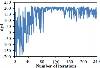
d) Variable C4
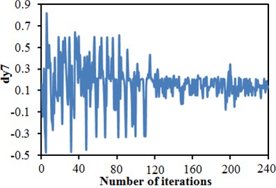
e) Variable C7
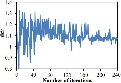
f) Variable C9
Fig. 25Iteration curves of optimization objectives
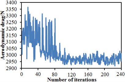
a) Aerodynamic drag
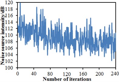
b) Dipole noise source intensity
In order to verify effectiveness of the improved NSGA-II algorithm in the paper, the traditional NSGA-II algorithm was used to conduct a multi-objective optimization for the head shape. Fig. 26 gives optimization objectives in the space when two kinds of optimization algorithms were adopted. In these figures, the lower left boundary was the Pareto front edge of the multi-objective aerodynamic optimization of the head shape; the square point “■” was the aerodynamic drag and dipole noise source corresponding to the initial streamline head shape. It is shown in these figures that, through a multi-objective optimization design on the streamline head shape of the high-speed train, the aerodynamic drag and dipole noise source of the high-speed train were reduced, and good optimization effects were obtained. It is found through comparison with the aerodynamic performance of the original streamline head shape that: through optimization with the traditional NSGA-II algorithm, the aerodynamic drag of the high-speed train could be most reduced by 4.54 %, and the dipole aerodynamic noise source could be most reduced by 4.95 dB; through optimization with the improved NSGA-II algorithm, the aerodynamic drag of the high-speed train could be most reduced by 6.74 %, and the dipole aerodynamic noise source could be most reduced by 8.34 dB. Obviously, the improved NSGA-II algorithm proposed in the paper has obvious advantages for the multi-objective optimization of the head shape. An acoustic model of the high-speed train was re-established according to optimized parameters; near-field and far-field aerodynamic noises of the high-speed train were computed and compared with original results, as shown in Fig. 27. It is shown in these figures that optimization effects were not obvious in low frequency bands; however, in mid-high frequency bands, the aerodynamic noise of the high-speed train was reduced obviously.
Fig. 26Pareto front edge of the optimization objective
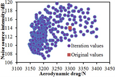
a) Traditional NSGA-II algorithm
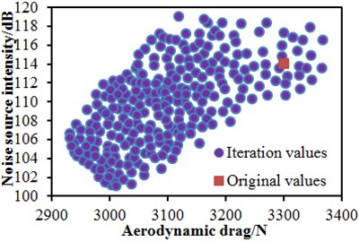
b) Improved NSGA-II algorithm
Fig. 27Reduction of near-field and far-field noises of the high-speed train
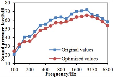
a) Near-field noises
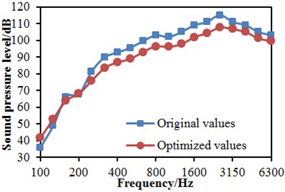
b) Far-field noises
7. Conclusions
Based on Lighthill acoustic theory, this paper adopted LES and FW-H acoustic models to conduct numerical computation for the aerodynamic noise of a high-speed train, analyzed the aerodynamic flow behavior, far-field and near-field aerodynamic noises of the high-speed train, and obtained the following conclusions:
1) Vortexes of head of the high-speed train were mainly striped. Horseshoe-shaped or hairpin vortexes were mainly in the area of tail train. In addition, vortexes were symmetrically distributed along the longitudinal symmetry plane of train.
2) The main aerodynamic noise source of the high-speed train was mainly distributed at the nose tip of head train. In addition, large turbulent kinetic energy was distributed in the streamlined position of head train. It could be seen that the streamlined position of head train was also the main aerodynamic noise source of the high-speed train. Fluid separation and recombination were main factors for the formation of aerodynamic noise of the high-speed train.
3) The dipole source of the high-speed train was mainly distributed in the position of head train. The maximum sound power level was linearly related to the logarithm of running speed. The maximum sound power level at the nose tip of head train was linearly related to 7.5th power of running speed; the maximum sound power level at the nose tip of tail train was linearly related to 6.7th power of running speed. Quadrupole noise was mainly distributed in the wake flow area of tail train.
4) When the high-speed train ran at the speed of 300 km/h, far-field sound pressure levels distributed along the longitudinal direction of train showed the following characteristics: The sound pressure level of aerodynamic noise of high-speed train gradually decreased along the flow direction of airflow. The sound pressure level of far-field aerodynamic noise reached a local maximum where there was a transition from the streamlined position of head train to the non-streamlined position of head train and from the non-streamlined position of tail train to the streamlined position of tail train. At the observation point z13, the maximum sound pressure level was 76.8 dB. The sound pressure level of head train was decreased by 3.2 dB most while the sound pressure level of tail train decreased by 2.9 dB most.
5) Computational results of sound radiation of aerodynamic noise of high-speed train showed: Dipole source on the surface of the high-speed train body gradually weakened its intensity with the increase of frequency, whose main energy was in the streamlined position of head train. At the same frequency, the radiation of dipole sources of train surface on the longitudinal symmetry plane was mainly within the range of included angle from 25° to 160° formed with the ground. The intensity of radiation in the direction of track was relatively weak. In addition, the maximum sound pressure level of radiation sound field decreased from 115 dB to 96 dB and showed a decreasing tendency when the frequency increased from 1000 Hz to 5000 Hz.
6) In order to verify effectiveness of the improved NSGA-II algorithm in the paper, the traditional NSGA-II algorithm was used to conduct a multi-objective optimization for the head shape. It is found through comparison with the aerodynamic performance of the original streamline head shape that: through optimization with the traditional NSGA-II algorithm, the aerodynamic drag of the high-speed train could be most reduced by 4.54 %, and the dipole aerodynamic noise source could be most reduced by 4.95 dB; through optimization with the improved NSGA-II algorithm, the aerodynamic drag of the high-speed train could be most reduced by 6.74 %, and the dipole aerodynamic noise source could be most reduced by 8.34 dB. Obviously, the improved NSGA-II algorithm proposed in the paper has obvious advantages for the multi-objective optimization of the head shape. Near-field and far-field aerodynamic noises of the high-speed train were computed and compared with original results. Optimization effects were not obvious in low frequency bands; however, in mid-high frequency bands, the aerodynamic noise of the high-speed train was reduced obviously.
References
-
Schetz J. A. Aerodynamics of high-speed trains. Annual Review of Fluid Mechanics, Vol. 33, Issue 1, 2001, p. 371-414.
-
Luo Q. L., Fang W. Reliable broadband wireless communication for high speed trains using baseband cloud. EURASIP Journal on Wireless Communications and Networking, Vol. 2012, 2012, p. 1-12.
-
Gawthorpe R. G. Train drag reduction from simple design changes. International Journal of Vehicle Design, Vol. 3, Issue 3, 1982, p. 263-274.
-
Wei W., Fan X., Song H., et al. Imperfect information dynamic stackelberg game based resource allocation using hidden Markov for cloud computing. IEEE Transactions on Services Computing, 2016, https://doi.org/10.1109/TSC.2016.2528246.
-
Mellet C., Létourneaux F., Poisson F., et al. High speed train noise emission: Latest investigation of the aerodynamic/rolling noise contribution. Journal of Sound and Vibration, Vol. 293, Issue 3, 2006, p. 535-546.
-
Brockie N. J. W., Baker C. J. The aerodynamic drag of high speed trains. Journal of Wind Engineering and Industrial Aerodynamics, Vol. 34, Issue 3, 1990, p. 273-290.
-
Poisson F. Railway Noise Generated by High-Speed Trains. Noise and Vibration Mitigation for Rail Transportation Systems. Springer, Berlin, Heidelberg, 2015, p. 457-480.
-
Thompson D. J., Latorre Iglesias E., Liu X., et al. Recent developments in the prediction and control of aerodynamic noise from high-speed trains. International Journal of Rail Transportation, Vol. 3, Issue 3, 2015, p. 119-150.
-
Shen Z. Y. Dynamic environment of high speed train and its distinguished technology. Journal of the China Railway Society, Vol. 28, Issue 4, 2006, p. 1-5.
-
Zhang W. H. Study on top-level design specifications of high speed trains. Journal of the China Railway Society, Vol. 34, Issue 9, 2012, p. 15-19.
-
Jin X. Key problems faced in high-speed train operation. Journal of Zhejiang University Science A, Vol. 15, Issue 12, 2014, p. 936-945.
-
Marié S., Ricot D., Sagaut P. Comparison between lattice Boltzmann method and Navier-Stokes high order schemes for computational aeroacoustics. Journal of Computational Physics, Vol. 228, Issue 4, 2009, p. 1056-1070.
-
Sassa T., Sato T., Yatsui S. Numerical analysis of aerodynamic noise radiation from a high-speed train surface. Journal of Sound and Vibration, Vol. 247, Issue 3, 2001, p. 407-416.
-
Takaishi T., Ikeda M., Kato C. Method of evaluating dipole sound source in a finite computational domain. The Journal of the Acoustical Society of America, Vol. 116, Issue 3, 2004, p. 1427-1435.
-
Takaishi T., Sagawa A., Nagakura K., et al. Numerical analysis of dipole sound source around high speed trains. The Journal of the Acoustical Society of America, Vol. 111, Issue 6, 2002, p. 2601-2608.
-
Li S. Y., Yang X. W. A mathematical model of the vehicle interior sound field. Journal of Vibration Engineering, Vol. 7, Issue 3, 1994, p. 275-279.
-
Liu H. G., Lu S. L. Calculation method of the aerodynamic noise around high speed vehicles. Journal of Traffic and Transportation Engineering, Vol. 2, Issue 2, 2002, p. 41-44.
-
Xia H., Gong Z., Lu S. L., Yao Z. Y. A research on calculating method of interior aerodynamic noise for high-speed automobile. Automotive Engineering, Vol. 25, Issue 1, 2003, p. 78-81.
-
Xia H., Gong Z., Lu S. L. Calculations about interior aerodynamic noise for high speed automobile by BEM. Journal of Jangsu University (Natural Science Edition), Vol. 24, Issue 1, 2003, p. 47-50.
-
Wang Y. P., Gu Z. Q., Yang X., Li W. P., Yuan Z. Q. Aerodynamic noise analysis and control for mini-car side view mirror. Journal of Aerospace Power, Vol. 24, Issue 7, 2009, p. 1577-1583.
-
Xiao Y. G., Tian H. Q., Zhang H. Prediction of interior aerodynamic noise of high speed train cab. Journal of Traffic and Transportation Engineering, Vol. 8, Issue 3, 2008, p. 10-14.
-
Yang F., Zheng B. L., He P. F. Numerical simulation on aerodynamic noise of power collection equipment for high speed trains. Computer Aided Engineering, Vol. 19, Issue 1, 2010, p. 44-47.
-
Zhu J., Hu Z., Thompson D. J. Flow behaviour and aeroacoustic characteristics of a simplified high-speed train bogie. Proceedings of the Institution of Mechanical Engineers, Part F: Journal of Rail and Rapid Transit, Vol. 230, Issue 7, 2016, p. 1642-1658.
-
Lee J., Cho W. Prediction of low-speed aerodynamic load and aeroacoustic noise around simplified panhead section model. Proceedings of the Institution of Mechanical Engineers, Part F: Journal of Rail and Rapid Transit, Vol. 222, Issue 4, 2008, p. 423-431.
-
Ikeda M., Suzuki M., Yoshida K. Study on optimization of panhead shape possessing low noise and stable aerodynamic characteristics. Quarterly Report of RTRI, Vol. 47, Issue 2, 2006, p. 72-77.
-
Liu J. L., Zhang J. Y., Zhang W. H. Numerical analysis on aerodynamic noise of the high speed train head. Journal of the China Railway Society, Vol. 33, Issue 9, 2011, p. 19-26.
-
Schmitt P., Poinsot T., Schuermans B., et al. Large-eddy simulation and experimental study of heat transfer, nitric oxide emissions and combustion instability in a swirled turbulent high-pressure burner. Journal of Fluid Mechanics, Vol. 570, 2007, p. 17-46.
-
Wolf P., Staffelbach G., Gicquel L. Y. M., et al. Acoustic and large eddy simulation studies of azimuthal modes in annular combustion chambers. Combustion and Flame, Vol. 159, Issue 11, 2012, p. 3398-3413.
-
Ding G., Tan Z., Wu J., et al. Indoor fingerprinting localization and tracking system using particle swarm optimization and Kalman filter. IEICE Transactions on Communications, Vol. 98, Issue 3, 2015, p. 502-514.
-
Wei W., Song H., Li W., et al. Gradient-driven parking navigation using a continuous information potential field based on wireless sensor network. Information Sciences, Vol. 408, 2017, p. 100-114.
-
Calaf M., Meneveau C., Meyers J. Large eddy simulation study of fully developed wind-turbine array boundary layers. Physics of Fluids, Vol. 22, Issue 1, 2010, p. 15110.
-
Huang S., Yang M. Z., Li Z. W. Aerodynamic noise numerical simulation and noise reduction of high-speed bogie section. Journal of Central South University (Science and Technology), Vol. 42, Issue 12, 2011, p. 3899-3904.
-
Williams J. E. F., Hawkings D. L. Sound generation by turbulence and surfaces in arbitrary motion. Philosophical Transactions of the Royal Society of London A: Mathematical, Physical and Engineering Sciences, Vol. 264, Issue 1151, 1969, p. 321-342.
-
Xiao P., Cowan C. F. N. MIMO detection schemes with interference and noise estimation enhancement. IEEE Transactions on Communications, Vol. 59, Issue 1, 2011, p. 26-32.
-
Xiao P., Sellathurai M., et al. Iterative multiuser detection and decoding for DS-CDMA system with space-time linear dispersion. IEEE Transactions on Vehicular Technology, Vol. 58, Issue 5, 2009, p. 2343-2353.
-
Shi Q. J., Chen Q. C., et al. Optimum linear block precoding for multi-point cooperative transmission with per-antenna power constraints. IEEE Transactions on Wireless Communications, Vol. 11, Issue 9, 2012, p. 3158-3169.
-
Zhang L., Zhang J. Y., Li T., Zhang W. H. Multi-objective aerodynamic optimization design for head shape of high-speed trains. Journal of Southwest Jiaotong University, Vol. 51, Issue 6, 2016, p. 1055-1063.
-
Yu M. G., Zhang J. Y., Zhang W. H. Multi-objective aerodynamic optimization design of the streamlined head of high-speed trains under crosswinds. Journal of Mechanical Engineering, Vol. 50, Issue 24, 2014, p. 122-129.
-
Hu H. G., Wu J. S. New constructions of codebooks nearly meeting the Welch bound with equality. IEEE Transactions on Information Theory, Vol. 60, Issue 2, 2014, p. 1348-1355.
-
Wu J. S., Bisio I., Gniady C., et al. Context-aware networking and communications: Part 1. IEEE Communications Magazine, Vol. 52, Issue 6, 2014, p. 14-15.
-
Yang K., Yang N., Xing C. W., et al. Space-time network coding with transmit antenna selection and maximal-ratio combining. IEEE Transactions on Wireless Communications, Vol. 14, Issue 4, 2015, p. 2106-2117.
-
Ge C., Sun Z. L., Wang N., et al. Energy management in cross-domain content delivery networks: a theoretical perspective. IEEE Transactions on Network and Service Management, Vol. 11, Issue 3, 2014, p. 264-277.
-
Han F. X., Zhao S. J., Zhang L., et al. Survey of strategies for switching off base stations in heterogeneous networks for greener 5G systems. IEEE Access, Vol. 4, 2016, p. 4959-4973.
Cited by
About this article

This Project was supported by National Natural Science Fund of China (Grant No. 51608049).
