Prediction of natural frequency of basalt fiber reinforced polymer (FRP) laminated variable thickness plates with intermediate elastic support using artificial neural networks (ANNs) method

Altabey, Wael A.

doi:10.21595/jve.2017.18209

Journal of Vibroengineering

Browse Journal

Submit article

Published: 15 August 2017

Check for updates

Prediction of natural frequency of basalt fiber reinforced polymer (FRP) laminated variable thickness plates with intermediate elastic support using artificial neural networks (ANNs) method

Wael A. Altabey¹

¹International Institute for Urban Systems Engineering, Southeast University, Nanjing, 210096, China

¹Department of Mechanical Engineering, Faculty of Engineering, Alexandria University, Alexandria, 21544, Egypt

Cite the article Download PDF

Downloads 1384

WoS Core Citations 17

CrossRef Citations 22

Abstract

The paper is focused on the application of artificial neural networks (ANNs) in predicting the natural frequency of basalt fiber reinforced polymer (FRP) laminated, variable thickness plates. The author has found that the finite strip transition matrix (FSTM) approach is very effective to study the changes of plate natural frequencies due to intermediate elastic support (IES), but the method difficulty in terms of, a lot of calculations with large number of iterations is the main drawback of the method. For training and testing of the ANN model, a number of FSTM results for different classical boundary conditions (CBCs) with different values of elastic restraint coefficients ( $K_{T}$ ) for IES have been carried out to training and testing an ANN model. The ANN model has been developed using multilayer perceptron (MLP) Feed-forward neural networks (FFNN). The adequacy of the developed model is verified by the regression coefficient ( $R^{2}$ ) and Mean Square error (MSE) It was found that the R2 and MSE values are 0.986 and 0.0134 for train and 0.9966 and 0.0122 for test data respectively. The results showed that, the training algorithm of FFNN was sufficient enough in predicting the natural frequency in basalt FRP laminated, variable thickness plates with IES. To judge the ability and efficiency of the developed ANN model, MSE has been used. The results predicted by ANN are in very good agreement with the FSTM results. Consequently, the ANN is show to be effective in predicting the natural frequency of laminated composite plates.

1. Introduction

Continuous laminated plates and laminated composite plates with intermediate stiffeners are one of very common in composite structures that used in many engineering fields such as aerospace, civil and marine industries.

Natural frequencies of laminated composite structures are the classical tools for the intelligent diagnosis of composite defects (e.g. fiber breakage, matrix cracks, de-bonding and delamination). Vibration response has become an important tool in Structural health monitoring (SHM) in the last decades, the natural frequencies of composite structure are extracted and analyzed under each damage scenario as damage detection and localization technique based on the changes in vibration parameters. In the recent years, several approaches to find the natural frequencies and the mode shapes of laminated composite plates became a field that has attracted a lot of interest in the scientific community.

In order to find the natural frequencies and the mode shapes for different boundary conditions with IES, a numerical approach or an approximate method must be used. Several researchers are attracted to vibration of plates with IES. FSTM is one of a semi-analytical methods are welcomed in the many literatures as an alternative to the exact solution. In our previous paper by Altabey [1], a semi-analytical method, the FSTM approach has been used to investigate the free vibration of basalt FRP laminated variable thickness rectangular plates with IES. Since all of the coefficients in the FSTM method can be obtained, a lot of calculations with large number of iterations must be performed to obtain a frequency parameters, i.e. the time of solutions will be increased, and the large amount of data are required to study the changes of plate natural frequencies due to IES. This is the main drawback of the method identified so far.

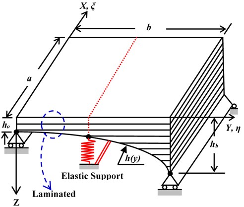
In the present study, the laminated composite plate shown in Fig. 1 has been modeled and analyzed using FSTM method. The laminated composite plate was manufactured using five symmetrically, angle-ply, laminates with the fiber orientations [45º/-45º/45º/-45º/45º] of basalt fiber and a polymer resin matrix. A predictive model for natural frequency in terms of fiber orientations is then developed using artificial neural networks. The developed model is tested with the FSTM data which were never used for developing the model. The FSTM results show that R2 and MSE are 0.986 and 0.0134 for train and 0.9966 and 0.0122 for test data respectively. Hence ANN model predicted results are in very good agreement with the FSTM results. Consequently, ANN are shown to be very effective in predicting the natural frequency of laminated composite plates under Four different CBCs are used in the analysis with different KT for IES.

Fig. 1The geometrical model of Basalt FRP laminated variable thickness rectangular plate with IES

2. Governing Equations

The normalized partial differential equation governing the vibration of symmetrically, angle-ply laminated, variable thickness, rectangular plates under the assumption of the classical deformation theory in terms of the plate deflection $w_{o} (x, y, t)$ using the non-Dimensional variables $ξ$ and $η$ is given by [1, 2]:

1

\begin{array}{l} ψ_{1} \frac{1}{a^{4}} W_{ξ ξ ξ ξ} + \frac{2 ψ_{2}}{h^{3} (η)} \frac{1}{a^{2} b} \frac{\partial h^{3} (η)}{\partial η} W_{ξ ξ η} + 2 ψ_{2} \frac{1}{a^{2} b^{2}} W_{ξ ξ η η} + ψ_{3} \frac{1}{a^{3} b} W_{ξ ξ ξ η} \\ + 4 ψ_{4} \frac{1}{a b^{3}} W_{ξ η η η} + \frac{1}{a b} \frac{4 ψ_{4}}{h^{3} (η)} \frac{\partial^{2} h^{3} (η)}{\partial η^{2}} W_{ξ η} + \frac{8 ψ_{4}}{h^{3} (η)} \frac{1}{a b^{2}} \frac{\partial h^{3} (η)}{\partial η} W_{ξ η η} \\ + \frac{1}{b^{2}} \frac{1}{h^{3} (η)} \frac{\partial^{2} h^{3} (η)}{\partial η^{2}} W_{η η} + \frac{1}{b^{4}} W_{η η η η} + \frac{2}{h^{3} (η)} \frac{1}{b^{3}} \frac{\partial h^{3} (η)}{\partial η} W_{η η η} = - \frac{m_{o}}{D_{22}} \frac{h_{o}^{2}}{h^{2} (η)} W_{t t}, \end{array}

where $β = a / b$ is the aspect ratio, also:

ξ = \frac{x}{a}, η = \frac{y}{b}, ψ_{1} = \frac{D_{11}}{D_{22}}, ψ_{2} = \frac{(D_{12} + 2 D_{66})}{D_{22}}, ψ_{3} = \frac{D_{16}}{D_{22}}, ψ_{4} = \frac{D_{26}}{D_{22}},

W_{ξ ξ ξ ξ} = \frac{\partial^{4} w_{o}}{\partial ξ^{4}}, W_{η η η η} = \frac{\partial^{4} w_{o}}{\partial η^{4}}, W_{ξ ξ η η} = \frac{\partial^{4} w_{o}}{\partial ξ^{2} \partial η^{2}},

W_{ξ ξ ξ η} = \frac{\partial^{4} w_{o}}{\partial ξ^{3} \partial η}, W_{η η η ξ} = \frac{\partial^{4} w_{o}}{\partial η^{3} \partial ξ}, W_{η η} = \frac{\partial^{2} w_{o}}{\partial t^{2}}, m_{o} = ρ h_{o}

$D_{i j}$ is the flexural rigidities matrix of the plate.

Since the treatment of IES conditions are the main objective of this paper we presented it in more details. At IES, $y = b / 2$ , the displacement must vanish and the moment must be continuous, i.e. [1]:

2

\frac{1}{b} {\frac{\partial w_{0}}{\partial η}|}_{η = 1^{-} / 2} = \frac{1}{b} {\frac{\partial w_{0}}{\partial η}|}_{η = 1^{+} / 2}

3. Finite strip transition matrix (FSTM) with artificial neural network (ANN) method

3.1. Finite strip transition matrix (FSTM) method

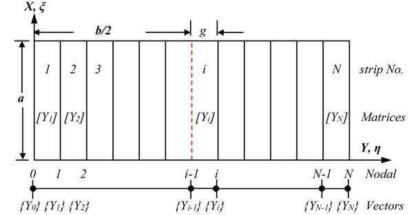
The method is made when such a shape function is not conveniently obtained in case of discussing the plate problems by series. The plate may be divided into N discrete longitudinal strips spanning between supports as shown in Fig. 2. By basic displacement interpolation functions may then be used to represent displacement field within and between individual strips.

For a plate striped in the $ξ$ -direction as shown in Fig. 2, the shape function $W (ξ, η, t)$ may be assumed in the form:

4

W (ξ, η, t) = \sum_{i = 0}^{N} X_{i} (ξ) Y_{i} (η) e^{i ω t},

where: $Y_{i} (η)$ is unknown function to be determined and $X_{i} (ξ)$ is chosen a priori, the basic function in $ξ$ -direction.

Fig. 2Finite strip simulation on plate

3.2. Artificial neural network (ANN) modeling

Artificial neural network (ANN) is an attractive inductive approach for modeling non-linear and complex systems without explicit physical representation and thus provides an alternative approach for modeling hydrologic systems. Artificial neural network was first developed in the 1940s. Generally speaking, ANNs are information processing systems. In recent decades, considerable interest has been raised over their practical applications. Training of artificial neural network enables the system to capture the complex and non-linear relationships that are not easily analyzed by using conventional methods such as linear and multiple regression methods and the network is built directly from experimental or numerical data by its self-organizing capabilities. Based on the different applications, various types of neural network with various algorithms have been employed to solve the different problems. In this work will be using the preferred ANN structures to predict the frequency parameter of presented numerical conditions.

3.2.1. ANN configuration

Since the ANN configuration has a great influence on the predictive quality, various arrangements have been considered in previous work. It is necessary to define a simple code to describe the ANN configuration, as follows:

5

\{N_{i n} {[\begin{array}{l} N_{h 1} & N_{h 2} \end{array}]}_{e} N_{o u t}\},

where $N_{i n}$ and $N_{o u t}$ are the element numbers of input and output parameters, respectively, and $e$ is the number of hidden layers. $N_{h 1}$ and $N_{h 2}$ are numbers of neurons in each hidden layer, respectively. For example, $\{7 {[21]}_{1} 1\}$ means a one hidden layer ANN with seven input and one output parameters, with the hidden layer containing 21 elements (neurons); $\{9 {[\begin{array}{l} 15 & 10 \end{array}]}_{2} 1\}$ denotes a nine input and one output ANN, with 15 and 10 neurons, respectively, in two hidden layers.

The powerful function of an ANN is due to the neurons within the hidden layers, as well as to the related interconnections. Networks are also sensitive to the number of neurons in their hidden layers. It is believed that an ANN can represent any reasonable relationship between input and output if the hidden layers have enough neurons. However, for the practical case, more hidden neurons bring more interconnections, which require, in turn, larger training datasets for learning the relationships. It is therefore always necessary to optimize the number of neurons of the ANN hidden layers, as demonstrated by Demuth and Beale [3].

3.2.2. Performance evaluation measures

It is very useful from the designer point of view to have a neural system aids to decide whether his suggested design is suitable or not by Compute the MSE from equation:

6

M S E = \sum \frac{{({(Ω)}_{n n} - Ω)}^{2}}{n},

where: ${(Ω)}_{n n}$ is the predicted frequency parameter from ANN, $Ω$ is the target or computed values from FSTM method of frequency parameter, and $n$ is the number of FSTM computed data values.

Thus, the performance index will either have one global minimum, depending on the characteristics of the input vectors. Local minimum is the minimum of a function over a limited range of input values. Local minimum is an unavoidable when the ANN is fitted. So, a local minimum may be good or bad depending on how close the local minimum is to the global minimum and how low an MSE is required. In any case, the method applied to solve this problem and descent the local minimum with momentum. Momentum allows a network to respond not only to the local gradient, but also to recent trends in the error surface. Without momentum a network may get stuck in a shallow local minimum.

The estimation performances of frequency parameter $(Ω)$ is evaluated by the lack of fit with the regression coefficient of the multiple determination $R^{2}$ ; $R^{2}$ is defined as:

7

R^{2} = 1 - \frac{\sum_{n} {({(Ω)}_{n n} - Ω)}^{2}}{\sum_{n} {(Ω)}^{2}} .

The value of $R^{2}$ is equal to or lower than 1.0. A higher value of $R^{2}$ implies a better fit. When the ANN shows a very good fit, $R^{2}$ approaches 1.0. A good fit of the ANN means that the ANN gives good estimations for the dielectric properties change used for the regression. Lower $R^{2}$ values means poorer estimations and the error band of the estimated result is wider.

3.3. Feed-forward neural networks (FFNN)

In this work we will use the suggested feed forward neural network, FFNN, to predict natural frequency of basalt FRP composite plate, because it has minimum mean square error (MSE), in composite structure applications [4, 5]. FFNN in general consist of a layer of input neurons, a layer of output neurons and one or more layers of hidden neurons [6]. Neurons in each layer are interconnected fully to previous and next layer neurons with each interconnection have associated connection strength or weight. The activation function used in the hidden and output layers neurons is nonlinear, where as for the input layer no activation function is used since no computation is involved in that layer. Information flows from one layer to the other layer in a feed-forward manner. Various functions are used to model the neuron activity such as liner transfer function ( $p u r e l i n (n)$ ), Tan-Sigmoid transfer function ( $t a n s i g (n)$ ) or Radial Basis (Gaussian) transfer functions ( $r a d b a s (n)$ ).

The training process is terminated either when the (MSE) between the observed data and the ANN outcomes for all elements in the training set has reached a pre-specified threshold or after the completion of a pre-specified number of learning epochs.

4. Results and discussion

In this work, The FSTM with ANNs techniques are used to predict the free vibration of the laminated composite plate shown in Fig. 1. The plate was manufactured using five symmetrically, angle-ply, laminates with the fiber orientations [ $θ$ / $- θ$ / $θ$ / $- θ$ / $θ$ ] is [45°/–45°/45°/–45°/45°] of basalt fiber and a polymer resin matrix. Physical and mechanical properties of the basalt FRP laminate composite plate are shown in Table 1.

Table 1Physical and mechanical properties of the basalt FRP

$E_{1}$	$E_{2} = E_{3}$	$G_{1} = G_{3}$	$G_{2}$	$υ_{1} = υ_{3}$	$υ_{2}$	$ρ$
96.74 GPa	22.55 GPa	10.64 GPa	8.73GPa	0.3	0.6	2700 kg/m³

The non-dimensional frequency parameter $Ω$ are addressed in form [1]:

8

Ω = \sqrt{\frac{m_{o} h (η) ω^{2} a^{4}}{h_{o} D_{22}}} .

The plate has linear deformation in thickness $h (y)$ woth non-dimensional form [1]:

9

h (η) = 1 + Δ η,

where: $Δ$ is the tapered ratio of plate given by $Δ = {(h}_{b} - h_{o}) / h_{o}$ , ( $h_{o}$ ) is the thickness of the plate at $η =$ 0 and ( $h_{b}$ ) is the thickness of the plate at $η =$ 1.

4.1. Convergence study and accuracy

In this subsection, the author has carried out for convergening the proposed method, first six frequencies are calculated and compared with available results in literatures [1]. He compared the computational results of FSTM method from previous work [1] with values available from literatures [7, 8] for E-glass/ epoxy, square ( $β =$ 1.0), uniform thickness ( $Δ =$ 0) plates with elastic foundation support, the mechanical properties of the plate material are $υ_{1} =$ $υ_{2} =$ 0.23, $D = E h^{3} / [12 (1 - υ^{2})]$ , and $D_{66} = (1 - υ) D / 2$ . Two different CBCs (SSSS and CCCC) are used in calculations, KT is taken equal to 500, 1390.2 for SSSS and CCCC respectively. In this study are addressed in form $Ω = {(ρ h ω^{2} a^{4} / D)}^{1 / 2}$ . He found the results by FSTM method are in a very close agreement with results in References [7, 8] and the convergence speed can be achieved with terms of series solution ( $N =$ 3 to 7).

4.2. Finite strip transition matrix (FSTM) results

In the present study, the numerical computations using FSTM approach is applied with an ANNs, which are combined to decrease detection effort to discern for different KT by minimizing the number of FSTM computations in order to keep save the time of calculations to a minimum. The method has successfully computations of the frequency parameter using only two different $K_{T}$ , the first one is located at $K_{T} =$ 50 the second is $K_{T} =$ 750, respectively, as shown in Table 2.

Table 2 presents the first six frequencies of the laminated composite plate shown in Fig. 1. The plate has the parameters of aspect ratio ( $β$ ) and thickness tapered ratio ( $Δ$ ) are 0.5. The Four different type of CBCs (SSSS, CCCC, SSFF and CCFF) and two different values of KT of IES are used in the calculations to study the changes of natural frequencies due to IES. The locations of the IES is at mid-line of the presented plate.

Table 2The first six frequencies of laminated, plate shown in Fig. 1 for two different values of KT, (Δ=0.5), (β=0.5)

	$K_{T}$	$Ω_{1}$	$Ω_{2}$	$Ω_{3}$	$Ω_{4}$	$Ω_{5}$	$Ω_{6}$
SSSS	50	22.1450	36.2210	53.5870	78.2360	105.5870	138.6970
SSSS	750	55.0692	69.1452	86.5112	111.1602	138.5112	171.6212
CCCC	50	28.4310	46.5025	68.7979	100.4437	135.5584	178.0668
CCCC	750	61.3551	79.4267	101.7221	133.3678	168.4826	210.9910
SSFF	50	12.2750	20.0773	29.7033	43.3663	58.5270	76.8799
SSFF	750	45.1992	53.0015	62.6275	76.2905	91.4511	109.8041
CCFF	50	19.5928	32.0466	47.4112	69.2194	93.4182	122.7123
CCFF	750	52.5170	64.9707	80.3353	102.1436	126.3424	155.6365

4.3. A feed-forward neural network (FFNN) design for predicting frequency parameters

A FFNN configuration in this case was $\{2 {[\begin{array}{l} 5 & 5 \end{array}]}_{2} 1\}$ , with tan-sigmoid neurons for the first layer while the second layer has pure linear ones. FFNN is trained by measuring values of $K_{T}$ , $θ$ to predict $Ω$ for four different CBCs are SSSS, CCCC, SSFF and CCFF. Determination of the hidden layer, in addition to the number of nodes in the input and output layers, for providing the best training results, was the initial phase of the training procedure. The target for MSE to be reached at the end of the simulations was 0.001. Since the second step was largely a trial-and-error process, and involved FFNNs with the number of hidden layer neurons more than five, it did not show any sizeable improvement in prediction accuracy. Thus, the number of neurons for the single hidden layer was selected as five neurons. Selection of the number of hidden layer neurons, with respect to the MSE term is shown in Fig. 3. In the first FFNN structure is applied for training the results data of FSTM. Fig. 4 shows the training performance of suggested FFNN.

Fig. 5 represents the comparison between the FSTM data and the feed-forward neural network FFNN predicted data ( $Ω$ ) for $K_{T} =$ 50 of four different CBCs are SSSS, CCCC, SSFF and CCFF. The results of this NN show much satisfactory predication quality for this case study. Fig. 6 shows the comparison between the FSTM data and the feed forward neural network FFNN expected (tested) data for $K_{T} =$ 750 of four different CBCs are SSSS, CCCC, SSFF and CCFF. From Fig. 6, it noted that the expected data from the suggested FFNN are applicable with the FSTM data.

Fig. 3Plot of MSE terms corresponding to the number of hidden layer neurons, used for selecting the optimum number of hidden layer neurons

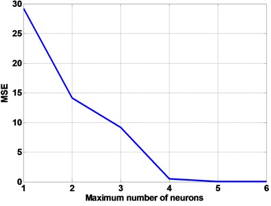
Fig. 4Training performance of suggested FFNN

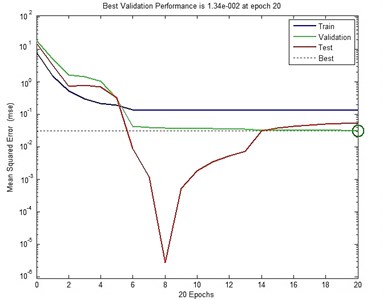
Fig. 5Comparison between the FSTM data and FFNN predicted data for Ω

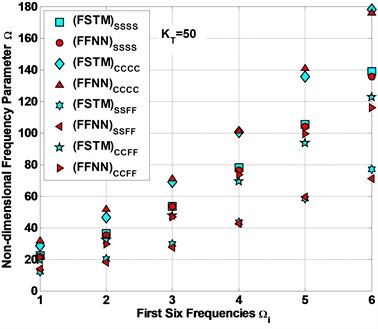
Fig. 6Comparison between the FSTM data and FFNN expected data for Ω

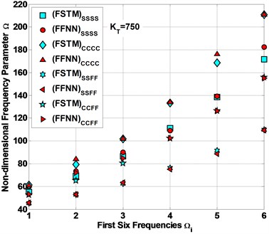
Fig. 7The performances of the present FFNN to predict data of Ω

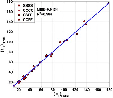
Fig. 8The performances of the present FFNN to expect data of Ω

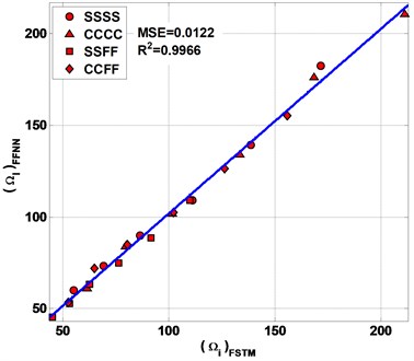
Table 3Mean square error (MSE) and regression coefficient (R2) values

Data	MSE	$R^{2}$
Predicted	0.0134	0.986
Expected	0.0122	0.9966

Table 3 and Figs. 7 and 8 represent the performances of the present FFNN by calculating the values of MSE and $R^{2}$ (see Eqs. (5, 6)) between FSTM data for both FFNN predicted and expected data for $Ω$ . As shown in Fig. 7 the value of MSE and $R^{2}$ between the FSTM and FFNN predicted data are 0.0134 and 0.986 respectively. From Fig. 8 the value of MSE and $R^{2}$ between the FSTM and FFNN expected data are 0.0122 and 0.9966 respectively.

4.4. The use of present FFNN for predicting non-FSTM data of non-dimensional frequency parameter $Ω$

The main goal of the artificial neural network design is predicting non- FSTM data. In this section we will use the suggested FFNN to predict some non- FSTM data not included in FSTM evaluation. It is selected to use seven different $K_{T}$ , for four types of CBCs (SSSS, CCCC, SSFF and CCFF). The previous parameters $K_{T}$ , $θ$ are the input vectors for artificial neural network, while the output is the signal vector is $Ω$ .

Fig. 9The FFNN predicted non-FSTM results of non-dimensional frequency parameter Ω

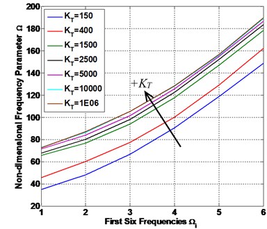
a) SSSS

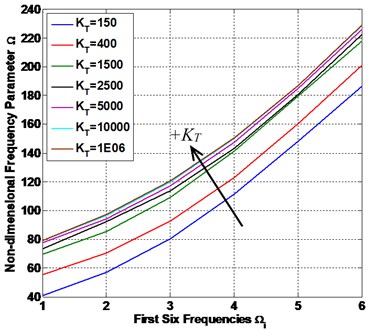
b) CCCC

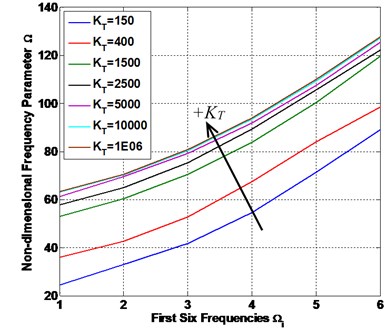
c) SSFF

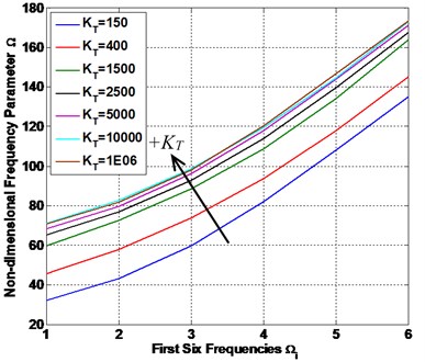
d) CCFF

Table 4The predicted non-FSTM results of the first six frequencies by FFNN

	$K_{T}$		$Ω_{1}$	$Ω_{2}$	$Ω_{3}$	$Ω_{4}$	$Ω_{5}$	$Ω_{6}$
SSSS	150	Ref [1]	34.6580	48.7340	66.1000	90.7490	118.1000	151.2100
	150	FFNN	34.8971	48.1343	66.6159	90.5891	118.8782	148.7286
	400	Ref [1]	45.8453	59.9213	77.2873	101.9363	129.2873	162.3973
	400	FFNN	45.8453	60.1268	77.2873	100.2624	129.2873	162.3973
	1500	Ref [1]	62.4709	76.5469	93.9129	118.5619	145.9129	179.0229
	1500	FFNN	65.5428	76.7674	93.799	117.6289	147.1225	178.4941
	2500	Ref [1]	67.5270	81.6030	98.9690	123.6180	150.9690	184.0790
	2500	FFNN	67.6715	80.0752	98.248	122.7383	152.2729	183.4709
	5000	Ref [1]	70.7832	84.8592	102.2252	126.8742	154.2252	187.3352
	5000	FFNN	71.5277	83.8535	101.5647	125.5413	154.9449	186.8396
	10000	Ref [1]	72.7065	86.7825	104.1485	128.7975	156.1485	189.2585
	10000	FFNN	72.8107	86.2942	105.2392	128.2564	156.1388	189.2703
	1E+06	Ref [1]	73.1195	87.1955	104.5615	129.2105	156.5615	189.6715
	1E+06	FFNN	72.6947	87.0396	105.4209	128.5854	156.8348	189.6596
CCCC	150	Ref [1]	40.9440	59.0155	81.3109	112.9567	148.0714	190.5798
	150	FFNN	41.0549	57.0992	80.3422	111.2997	148.2179	186.4952
	400	Ref [1]	52.1313	70.2028	92.4983	124.1440	159.2587	201.7672
	400	FFNN	55.4754	70.442	92.6468	123.0928	160.6131	201.1848
	1500	Ref [1]	68.7569	86.8284	109.1239	140.7696	175.8843	218.3928
	1500	FFNN	69.7659	85.3865	109.1148	141.4497	179.6854	218.0006
	2500	Ref [1]	73.8130	91.8845	114.1800	145.8257	180.9404	223.4489
	2500	FFNN	73.4808	92.2119	113.7449	143.3314	180.9021	222.5692
	5000	Ref [1]	77.0692	95.1407	117.4361	149.0819	184.1966	226.7050
	5000	FFNN	77.8273	94.092	117.0825	147.6263	184.9599	226.1968
	10000	Ref [1]	78.9925	97.0640	119.3594	151.0052	186.1199	228.6283
	10000	FFNN	79.3118	96.3864	119.7441	150.1071	187.0576	228.5796
	1E+06	Ref [1]	79.4055	97.4770	119.7724	151.4182	186.5329	229.0413
	1E+06	FFNN	79.1422	97.2499	120.7791	150.5119	186.7872	229.1948
SSFF	150	Ref [1]	24.7880	32.5903	42.2163	55.8793	71.0400	89.3929
	150	FFNN	24.4094	32.9047	41.7941	54.6268	71.2814	89.0171
	400	Ref [1]	35.9753	43.7777	53.4036	67.0666	82.2273	100.5802
	400	FFNN	35.9713	42.5469	52.8278	67.4484	83.9108	98.563
	1500	Ref [1]	52.6009	60.4033	70.0293	83.6922	98.8529	117.2058
	1500	FFNN	52.904	60.2689	70.3874	83.7121	100.3213	119.6639
	2500	Ref [1]	57.6570	65.4594	75.0853	88.7483	103.9090	122.2619
	2500	FFNN	57.9028	64.964	75.361	89.2589	105.6161	122.2164
	5000	Ref [1]	60.9132	68.7155	78.3415	92.0045	107.1652	125.5181
	5000	FFNN	61.3157	69.5938	79.1805	91.7539	107.5848	125.4066
	10000	Ref [1]	62.8365	70.6388	80.2648	93.9278	109.0885	127.4414
	10000	FFNN	63.0778	70.2994	80.2805	93.3565	109.3353	127.2809
	1E+06	Ref [1]	63.2495	71.0518	80.6778	94.3408	109.5015	127.8544
	1E+06	FFNN	63.3054	70.5596	80.69	93.9744	110.0274	127.6158
CCFF	150	Ref [1]	32.1058	44.5596	59.9242	81.7324	105.9312	135.2253
	150	FFNN	32.1827	43.2269	59.686	81.9174	108.2676	135.0946
	400	Ref [1]	43.2931	55.7469	71.1115	92.9197	117.1185	146.4127
	400	FFNN	45.562	57.8813	73.8431	93.8403	117.8631	145.3086
	1500	Ref [1]	59.9187	72.3725	87.7371	109.5453	133.7442	163.0383
	1500	FFNN	59.6275	72.4773	88.4423	108.7844	134.0482	163.8665
	2500	Ref [1]	64.9748	77.4286	92.7932	114.6014	138.8002	168.0944
	2500	FFNN	65.0645	76.7108	92.8809	114.0148	139.5554	167.6554
	5000	Ref [1]	68.2310	80.6848	96.0494	117.8576	142.0564	171.3505
	5000	FFNN	68.3337	79.7057	96.0889	117.8545	143.8554	171.2413
	10000	Ref [1]	70.1543	82.6081	97.9727	119.7809	143.9797	173.2738
	10000	FFNN	70.9017	82.7021	98.6556	119.3321	144.5419	173.0477
	1E+06	Ref [1]	70.5673	83.0211	98.3857	120.1939	144.3927	173.6868
	1E+06	FFNN	70.6424	81.6968	98.1541	120.3744	146.7246	173.5624

Fig. 10The performances of the present FFNN to predicted non-FSTM results of non-dimensional frequency parameter Ω

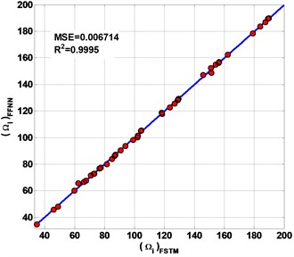
a) SSSS

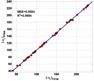
b) CCCC

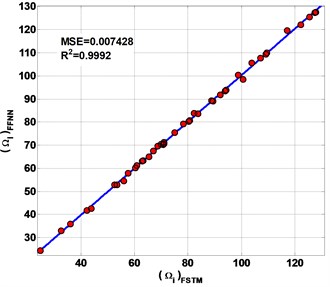
c) SSFF

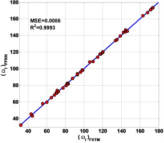
d) CCFF

Fig. 9 shows the FFNN predicted results of the first six frequencies of the laminated composite plate are presented in this study. The plate has $β =$ 0.5 and $Δ =$ 0.5 with four different types of CBCs.

The predicted non-FSTM results of the first six frequencies by FFNN and a comparison with the previous work results in literature of FSTM method by Altabey [1] are presented in Table 4. As a result, a FFNN gave good prediction for non-FSTM data even for extrapolations $Ω$ in presented laminated composite plate.

From Table 4 and Fig. 9, we can see, the first six frequencies increase with the increasing of the value of $K_{T}$ and we are observed that the gap between values of frequencies in the small $K_{T}$ and next values of $K_{T}$ are higher than the gap between values of frequencies in the large $K_{T}$ , and the frequencies at high values of $K_{T}$ are almost constant, for all conditions (SSSS, CCCC, SSFF and CCFF). On the other hand, the fully clamped (CCCC) and semi-simply supported (SSFF) condition have the higher and lower values of frequencies respectively and the other two conditions (SSSS) and (CCFF) are lie between them with an intermediate value. This conclusion was found in other work [1].

$R^{2}$ of non-FSTM results are 0.9995, 0.9994, 0.9992 and 0.9993 for SSSS, CCCC, SSFF and CCFF plate respectively. All of the predicting results are plotted on the diagonal line (Fig. 10) to observe the performances of the present FFNN to predict non-FSTM of $Ω$ . The MSE is defined of the predicted non- FSTM. The MSE is of non-FSTM results are 0.006714, 0.0084, 0.007428 and 0.0086 for SSSS, CCCC, SSFF and CCFF plate respectively.

5. Conclusions

The natural frequency values were found by analyses which were done of basalt FRP laminated variable thickness rectangular plates with IES by FSTM method and ANNs algorithm, which are combined to decrease computational effort to discern natural frequency in basalt FRP laminated composite plates, in order to save the time of the FSTM computational data to a minimum with high accuracy and easy. Based on the FSTM results and the results predicted by artificial neural networks, the following conclusions are drawn for laminated composite material plates.

1) The FFNN model has been developed by considering the $K_{T}$ and ply angle ( $θ$ ) as the input for predicting $Ω$ . The developed FFNN model could predict $Ω$ with the $R^{2}$ and MSE are 0.986 and 0.0134 for training data set and 0.9966 and 0.0122 for test data respectively.

2) The FFNN model could predict non-FSTM of $Ω$ with $R^{2}$ of non-FSTM results are 0.9995, 0.9994, 0.9992 and 0.9993 for SSSS, CCCC, SSFF and CCFF plate respectively. The MSE is defined of the predicted non-FSTM. The MSE is of non-FSTM results are 0.006714, 0.0084, 0.007428 and 0.0086 for SSSS, CCCC, SSFF and CCFF plate respectively.

3) The ANN predicted results are in very good agreement with the FSTM results.

References

Altabey W. A. Free vibration of basalt FRP laminated variable thickness plates with intermediate elastic support using finite strip transition matrix (FSTM) method. Journal of Vibroengineering, Vol. 19, Issue 4, 2017, (in Press).

Publisher
Chakraverty S. Vibration of Plates. CRC Press, Taylor and Francis Group, 2009.

Publisher
Demuth H., Beale M. Neural Network Toolbox User’s Guide for use with MATLAB Version 4.0. The Math Works, Inc., 2000.

Search CrossRef
Al-Tabey W. A. The Fatigue Behavior of Woven-Roving Glass Fiber Reinforced Epoxy under Combined Bending Moment and Hydrostatic Pressure. Ph.D. Theses, Alexandria University, Egypt, 2015.

Search CrossRef
Altabey W. A. Fatigue life prediction for carbon fiber/epoxy laminate composites under spectrum loading using two different neural network architectures. International Journal of Sustainable Materials and Structural Systems, 2017, (in Press).

Publisher
Skapura D. Building Neural Networks. ACM Press, Addison-Wesley Publishing Company, New York, 1996.

Search CrossRef
Zhou D., Cheung Y. K., Lo S. H., Au F. T. K. Three dimensional vibration analysis of rectangular thick plates on Pasternak foundation. International Journal of Numerical Methods in Engineering, Vol. 59, 2004, p. 1313-1334.

Publisher
Ferreira J. M., Roque C. M. C., Neves A. M. A., Jorge R. M. N., Soares C. M. M. Analysis of plates on Pasternak foundations by radial basis functions. Journal of Computational Mechanics, Vol. 46, 2010, p. 791-803.

Publisher

Cited by

Proceedings of the 4th International Conference on Advances in Civil and Ecological Engineering Research

Weixing Hong | Mohammad Noori | Hanqing Jiang | Yuhan Liu | Wael A. Altabey

(2023)

Proceedings of the 4th International Conference on Advances in Civil and Ecological Engineering Research

(2023)

Third International Conference on Computer Vision and Information Technology (CVIT 2022)

(2023)

Experimental and Computational Analysis of Free In-Plane Vibration of Curved Beams

Nupur Mohanty | Suvendu Kumar Sasmal | Uttam Kumar Mishra | Shishir Kumar Sahu

(2023)

Free vibration of axially or transversely graded beams using finite-element and artificial intelligence

Sefa Yildirim

(2022)

Finite Element and Neural Network Based Predictive Model to Determine Natural Frequency of Laminated Composite Plates with Eccentric Cutouts under Free Vibration

Mohamed Rida Seba | Said Kebdani

(2022)

The Damage Identification in Laminated Composite Plate under Fatigue Load through Wavelet Packet Energy Curvature Difference Method

Wael A. Altabey

(2022)

Proceedings of the 4th International Conference on Intelligent Science and Technology

(2022)

2022 International Conference on Electrical, Computer, Communications and Mechatronics Engineering (ICECCME)

Wael A. Altabey | Sallam A. Kouritem | Mohammed I. Abouheaf | Nabil Nahas

(2022)

2022 International Conference on Electrical, Computer, Communications and Mechatronics Engineering (ICECCME)

Wael A. Altabey | Sallam A. Kouritem | Mohammed I. Abouheaf | Nabil Nahas

(2022)

Ultra-broadband natural frequency using automatic resonance tuning of energy harvester and deep learning algorithms

Sallam A. Kouritem | Wael A. Altabey

(2022)

Selecting optimum levels of wavelet multi‐resolution analysis for time‐varying signals in structural health monitoring

Ahmed Silik | Mohammad Noori | Wael A. Altabey | Ramin Ghiasi

(2021)

Deep Learning-Based Crack Identification for Steel Pipelines by Extracting Features from 3D Shadow Modeling

(2021)

Reaching law based sliding mode control for a frame structure under seismic load

Ying Zhao | Mohammad Noori | Wael A. Altabey

(2021)

Parameter identification and dynamic response analysis of a modified Prandtl–Ishlinskii asymmetric hysteresis model via least-mean square algorithm and particle swarm optimization

Tianyu Wang | Mohammad Noori | Wael A Altabey | Mojtaba Farrokh | Ramin Ghiasi

(2021)

Applying deep learning and wavelet transform for predicting the vibration behavior in variable thickness skew composite plates with intermediate elastic support

Wael A. Altabey

(2021)

Experimental and Numerical Assessment on Seismic Performance of Earth Adobe Walls

Zele Li | Mohammad Noori | Wael A. Altabey

(2021)

Identification of cracks in an Euler–Bernoulli beam using Bayesian inference and closed-form solution of vibration modes

Tianyu Wang | Mohammad Noori | Wael A. Altabey

(2020)

A Comparison of Three Different Methods for the Identification of Hysterically Degrading Structures Using BWBN Model

Ying Zhao | Mohammad Noori | Wael A. Altabey | Taher Awad

(2019)

Deep Learning-Based Damage, Load and Support Identification for a Composite Pipeline by Extracting Modal Macro Strains from Dynamic Excitations

Ying Zhao | Mohammad Noori | Wael A. Altabey | Ramin Ghiasi | Zhishen Wu

(2018)

Fatigue damage identification for composite pipeline systems using electrical capacitance sensors

Ying Zhao | Mohammad Noori | Wael A Altabey | Zhishen Wu

(2018)

High performance estimations of natural frequency of basalt FRP laminated plates with intermediate elastic support using response surfaces method

Wael A. Altabey

(2018)

About this article

Received

26 January 2017

Accepted

03 May 2017

Published

15 August 2017

SUBJECTS

Modal analysis and applications

DOI

https://doi.org/10.21595/jve.2017.18209

Keywords

artificial neural networks (ANNs)

free vibration

finite strip transition matrix

variable thickness plate

basalt FRP

This is an open access article distributed under the Creative Commons Attribution License, which permits unrestricted use, distribution, and reproduction in any medium, provided the original work is properly cited.

Previous article in issue Previous Next article in issue Next

Research article

2023 10 20

Damage detection in variable temperature conditions using artificial intelligence

Alexandra-Teodora Aman, Cristian Tufisi, Gilbert-Rainer Gillich, Tiberiu Manescu

Research article

2023 08 02

A novel model for predicting tenacity and unevenness of ring-spun yarn: a special case in textile engineering

Valentinus Galih Vidia Putra, Juliany Ningsih Mohamad

Research article

2022 05 16

Effectiveness analysis of structural anomaly diagnosis based on ANN model

Zhigang Ruan, Zuguang Ying

Research article

2021 02 06

Applying deep learning and wavelet transform for predicting the vibration behavior in variable thickness skew composite plates with intermediate elastic support

Wael A. Altabey

W. A. Altabey, “Prediction of natural frequency of basalt fiber reinforced polymer (FRP) laminated variable thickness plates with intermediate elastic support using artificial neural networks (ANNs) method,” Journal of Vibroengineering, Vol. 19, No. 5, pp. 3668–3678, Aug. 2017, https://doi.org/10.21595/jve.2017.18209

Copy Extrica

Copied to clipboard!

TY  - JOUR
DO  - 10.21595/jve.2017.18209
UR  - https://doi.org/10.21595/jve.2017.18209
TI  - Prediction of natural frequency of basalt fiber reinforced polymer (FRP) laminated variable thickness plates with intermediate elastic support using artificial neural networks (ANNs) method
T2  - Journal of Vibroengineering
AU  - Altabey, Wael A.
PY  - 2017
DA  - 2017/08/15
PB  - JVE International Ltd.
SP  - 3668-3678
IS  - 5
VL  - 19
SN  - 1392-8716
ER  - 

Copy Ris

Copied to clipboard!

@article{Altabey_2017,
	doi = {10.21595/jve.2017.18209},
	url = {https://doi.org/10.21595/jve.2017.18209},
	year = 2017,
	month = {aug},
	publisher = {{JVE} International Ltd.},
	volume = {19},
	number = {5},
	pages = {3668--3678},
	author = {Wael A. Altabey},
	title = {Prediction of natural frequency of basalt fiber reinforced polymer ({FRP}) laminated variable thickness plates with intermediate elastic support using artificial neural networks ({ANNs}) method},
	journal = {Journal of Vibroengineering}
}

Copy Bibtex

Copied to clipboard!

[1]W. A. Altabey, “Prediction of natural frequency of basalt fiber reinforced polymer (FRP) laminated variable thickness plates with intermediate elastic support using artificial neural networks (ANNs) method,” Journal of Vibroengineering, vol. 19, no. 5, pp. 3668–3678, Aug. 2017, doi: 10.21595/jve.2017.18209.

Copy IEEE

Copied to clipboard!

Altabey, Wael A. “Prediction of Natural Frequency of Basalt Fiber Reinforced Polymer (FRP) Laminated Variable Thickness Plates with Intermediate Elastic Support Using Artificial Neural Networks (ANNs) Method.” Journal of Vibroengineering 19, no. 5 (August 15, 2017): 3668–78. https://doi.org/10.21595/jve.2017.18209.

Copy Chicago

Copied to clipboard!

Prediction of natural frequency of basalt fiber reinforced polymer (FRP) laminated variable thickness plates with intermediate elastic support using artificial neural networks (ANNs) method

Abstract

1. Introduction

2. Governing Equations

3. Finite strip transition matrix (FSTM) with artificial neural network (ANN) method

3.1. Finite strip transition matrix (FSTM) method

3.2. Artificial neural network (ANN) modeling

3.2.1. ANN configuration

3.2.2. Performance evaluation measures

3.3. Feed-forward neural networks (FFNN)

4. Results and discussion

4.1. Convergence study and accuracy

4.2. Finite strip transition matrix (FSTM) results

4.3. A feed-forward neural network (FFNN) design for predicting frequency parameters

4.4. The use of present FFNN for predicting non-FSTM data of non-dimensional frequency parameter Ω

5. Conclusions

References

Cited by

About this article

Related Articles

4.4. The use of present FFNN for predicting non-FSTM data of non-dimensional frequency parameter $Ω$