Abstract
Most complex engineering structures are three-dimensional in practice. The process of one-dimensional extending to three-dimensional is a challenge that must be conquered by Operational Modal Analysis (OMA) methods when these methods are applied to complex engineering applications supported by scientific researches. This study put forward a new three-dimensional structure OMA method based on Second-Order Blind Identification (SOBI) and general reversion of least square. Firstly, modal coordinates decomposition of one-dimensional structural vibration response signal with SOBI. Secondly, the reasons that modal parameters identified by SOBI including energy uncertainty, order uncertainty and modal missing are explained in theory. Thirdly, the SOBI algorithm is used to decompose the response signals of displacement of a direction whose vibration response is the largest, then the other two directions are calculated by using the least square generalized inverse algorithm, and the modal parameters of three-dimensional structures are identified by the matrix assembly method. Numerical simulation results in a cylindrical shell demonstrated that this novel method is practical and effective by applied to practice in OMA of three-dimensional structures, and robustness to Gauss measurement noise disturbances.
1. Introduction
Unlike experimental modal analysis, Operational Modal Analysis (OMA) extracts modal parameters (including mode shapes, natural frequencies and damping ratios) only from vibration response signals when the structures are working condition [1]. There are some distinct advantages to adopt this approach: 1) The structure bears ambient excitation not artificial excitation; 2) The identified modal parameters, which can truly reflect on the dynamic characteristics of working structures, conforms to the real work and boundary condition. Therefore, OMA is more suitable for practical engineering applications and has great significance in areas of quality control, health monitoring and damage diagnosis [2-5].
A variety of methods about OMA are developed all over the world. Considering both categories: the domain of frequency and the domain of time [6], the blind source separation technique belongs to the latter [7, 8]. What is more, it is demonstrated that there is a one-to-one correspondence between the vibration modes and the mixing matrix in free and random vibrations of weakly damped systems [9]. Second-Order Blind Identification (SOBI) is a way of the blind source separation technique [10-11], and it has been applied to the field of OMA [12-14] since 2007. However, the research on three-dimensional structures of output-only modal analysis with the blind source separation technique is quite rare [15].
As three-dimensional structures are more complex, the process of modal analysis of three-dimensional structure is a challenge and will be conquered by OMA methods, when the methods are applied to engineering applications supported by scientific researches. Thus, this study proposes a new OMA method based on SOBI of three-dimensional structures. Firstly, this new method takes advantages of the SOBI algorithm to decompose the response signals of displacement of the largest one direction. Secondly, the other two directions are calculated by using the general reversion of least square algorithm, and finally the modal parameters of three-dimensional structures are identified by the matrix assembly method.
The remainder of this study is structured as follows: Section 2 describes the principle of SOBI, and applies SOBI to OMA of three-dimensional structure in Section 3. The identification results of a cylindrical shell and analysis are focus in Section 4. Finally, the conclusions and outlooks are outlined in Section 5.
2. SOBI for OMA of one-dimensional structures
2.1. The model of blind source separation
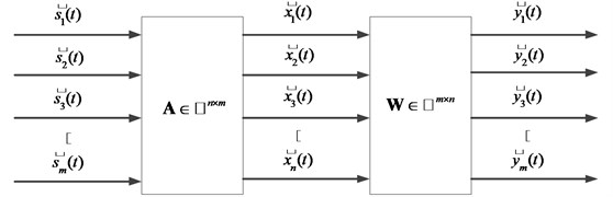
Supposing that observed signals mixed by several unobserved signals , the linear blind source separation model under the condition of non-noise is expressed as:
where, is a mixing matrix. In the present of measurement noises, the source identification model can be expressed as:
In order to recover source signals from observed mixing signals , it is necessary to find a separated matrix to meet the following equation:
where, is an estimation matrix of , Fig. 1 shows the principle of blind source separation.
Fig. 1The model of blind source separation
2.2. Using SOBI to solve blind source separation model
The main idea of the blind source separation is that recovering the unobserved source signals from multiple observed mixing signals without any prior information. SOBI is a blind source separation technique, which is different from independent component analysis [16]. By using joint diagonalization of a set of covariance matrices, SOBI can estimate the separated matrix effectively [10].
Second order blind identification mainly uses the joint diagonalization of a set of covariance matrices to estimate source signals accurately. There are two hypotheses: The mixing matrix is a column full rank matrix and the sources are not related to each other.
According to the hypotheses, the whiten matrix is calculated by eigenvalue decomposition as below:
where is a diagonal matrix composed by eigenvalues , is a eigenvector matrix of the covariance matrix . Thus, the observed matrix is preprocessed to :
When the matrix is a whiten matrix, the covariance matrix of is a unit matrix, and the second-order correlation between each component has been removed.
The set of covariance matrices is estimated as follows:
where is a fixed time delay.
For all the , using joint diagonalization algorithm, the orthogonal matrix is estimated:
where is a diagonal matrix.
Therefore, the source signals can be estimated as :
And the separated matrix is:
An estimation matrix of mixing matrix is:
2.3. Uncertainty factors in using SOBI to solve blind source separation model
It is easy to find some inevitable ambiguity or uncertainty factors from Eq. (1), which are summarized as followings:
a) The variance of the separated signal is uncertain.
Suppose is a diagonal matrix, the linear instantaneous mixture modal can be expressed as:
So, the amplitude of separated signal is inconsistent with the amplitude of source signals.
b) The order of the separated signal is uncertain.
Suppose is a permutation matrix, the linear instantaneous mixture modal can be expressed as:
where is a new source signals matrix after reordering and is a new mixing matrix.
The reason is that it is impossible to determinate specific values of the mixing matrix and source signals simultaneously without any prior knowledge.
c) The number of separated components is uncertain
It is hard to identify and separate independent components, if the contribution of independent components is not sufficient. So, without any prior knowledge, to determine the number of separated components or sources by the SOBI algorithm is difficult.
2.4. Modal coordinates decomposition of one-dimensional structural vibration response signal
OMA extracts modal parameters (including mode shapes, natural frequencies and damping ratios) only from response signals when the structures at working condition. For -degree of freedom time-invariant vibration systems, the kinetic equation is:
In Eq. (13), , , represent the mass matrix, the damping matrix and the stiffness matrix, respectively. is an external excitation, as well as is a displacement matrix, and are the first derivative and the second derivative of respectively.
For proportional damped vibration systems under ambient excitation, it’s random vibration response that can be decomposed in modal coordinates:
In Eq. (14), represents modal shape matrix making a series of mode shapes and is the vector matrix composed of each order modal response . Through the modal response, the mode frequency and modal damping ratio can be calculated.
By the way, normalized modal shapes and the modal response matrix meet:
where represents expectation, and is a diagonal matrix whose size is .
2.5. OMA for one-dimensional structures by SOBI and its uncertainty factors
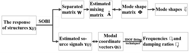
According to the mode theory, it is well known that each of the modal coordinates vector is independent. Combining with the SOBI algorithm, the response of structures decomposes into mode coordinate vectors and a mode shape matrix. Modal coordinates vectors can be regarded as source signals, and responses of systems can be recognized as observed signals, as well as the modal shape matrix is the mixing matrix. Therefore, SOBI can identify the modal parameters, and the process of identifying as showed in Fig. 2.
Fig. 2The process of identifying modal parameters by SOBI
On account of three assumptions of the SOBI method, the identified modal parameters have the following characteristics.
Every order of the modal shape has the different amplitude. In case of the SOBI method, the energy of separation matrix is not unique, and separated components also lose amplitude information. Unlike the principal component analysis method [17], the SOBI method cannot get the contribution ratio information of each modal. The modal shape is a relative quantity rather than an absolute value. So, in order to compare the modal shape with the real modal shape, the separation matrix and the modal shape identified by the SOBI method should be normalized.
The order of modal parameter identified by SOBI is uncertain. Modals identified by the SOBI method are not in accordance with the order from small to large. In fact, the first separated output modal is the one whose independence is the strongest rather than the first order modal parameter. Therefore, in order to compare natural frequencies with real natural frequencies, modal parameters need to be reordered by modal frequencies.
It is hard to identify and separate independent components, and to determine the numbers of modal parameters if the contribution of independent components is not sufficient. So, in the SOBI algorithm based output-only modal analysis, if the modal parameter is a small contribution to independence, the SOBI method may barely identify them and will cause modal parameters missing.
3. SOBI for OMA of three-dimensional structures
3.1. Problems and differences in OMA for one-dimensional to three-dimensional structures
Actual engineering structures are three-dimensional. From one-dimensional to three-dimensional, it takes a big step from scientific researches to engineering applications of modal analysis based on a series of blind source separation methods.
The matrix assembles: the vibration matrix of one-dimensional structures is a one-dimensional vector, the proportion of the value of each modal makes sense, but the amplitude of the modal does not make any sense. And the vibration matrix of the three-dimensional structure is combined by three directions , and . Each direction of the scale factor and the modulus ratio should stay the same, otherwise it becomes a one-dimensional vibration mode of three directions, rather than a three-dimensional vibration mode of structures. How to carry out this process is a big challenge.
As the three-dimensional structures are more complex, it is inevitable that the errors of the identified modal parameters will be the greater than the identified modal parameters in one-dimensional structures.
3.2. Modal coordinates decomposition of three-dimensional structural vibration response signals
For complex three-dimensional continuous systems under ambient excitation, its random response in time domain can be decomposed in modal coordinates:
where , , are the th () mode shape vector of ,and direction. is the th modal coordinate response which contains the information of the modal natural frequency.
In finite element analysis and experimental analysis, the three-dimensional systems are discretized to test points, and the time is discretized to number of sampling points, and . Therefore, the vibration response in the domain of time can be approximated as:
where is the number of modal truncation calculated by finite element analysis. of three directions are the same, so the modal coordinate response just should be calculated only once.
3.3. Right pseudo inverse and its general reversion the minimal norm solution of least square
Modal coordinates responses are the same in three directions. is the discretized number, and is the the number of modal truncation. So and , the matrix is reversible. The right pseudo inverse matrix defined as [19]:
where the right pseudo inverse matrix meets , the right pseudo inverse matrix is uniquely determined and right pseudo inverse is associated with its general reversion the minimal norm solution of least square.
After decomposing the response in one direction based on the SOBI modal analysis algorithm, this study requires to take use of the mode shape of the first direction, and calculates the modal parameters of the other two directions by the general reversion of least square algorithm.
The least squares generalized inverse method is the unbiased optimal estimate of the sum of squares of errors and the minimum sense [19, 20]. Supposing the vibration response direction is the largest, the mode shape matrix and the modal coordinate response of direction is known, according to Eq. (18), the vibration response of direction:
Multiplied by on both sides of Eq. (20):
So, the mode shape matrix of direction can be expressed as:
In the same way, the mode shape matrix of direction also can be got:
3.4. OMA for three-dimensional structures by SOBI and general reversion of least square
The select of a direction decomposed by the SOBI algorithm: in the first place, one direction of three-dimensional structures is decomposed by SOBI, however if selecting the different directions to decompose, it will affect the final effect of modal parameters. So, which directions are decomposed needs to be explained theoretically and demonstrated by experiments.
The modal response matrix returns into other two directions: since the modal response is the same in three directions, decomposing the response of one direction based on SOBI modal analysis algorithm which requires to return into the other two directions. The modal response is a matrix. How to return into the other directions? In practice, the response of other two directions is multiplied by the inverse of the modal response matrix.
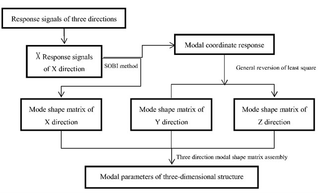
In order to identify operational modal parameters of three-dimensional structures, a strategy is adopted as below and the process of OMA for three-dimensional structures is shown in Fig. 3 below (Supposing that vibration response of direction is largest).
1) The purposed method takes advantages of SOBI algorithm to decompose a direction of the response signals of displacement which vibration response is the largest. Supposing the vibration response direction is the largest, we can get the mode shape matrix and modal coordinate response of direction.
2) The purposed method calculates the mode shape matrix of other two directions by using the general reversion of least square algorithm. The mode shape matrix of direction can be calculated with Eq. (22) and the mode shape matrix of direction can be calculated with Eq. (23).
3) The modal parameters of three-dimensional structures are identified by the matrix assembly method. In other words, is the th mode shape of three-dimensional structures, and is the th modal coordinates response.
Fig. 3Process of OMA for three-dimensional structure
4. Operational modal identification Simulation verification of three-dimensional structures
4.1. Simulation data generation of three-dimensional structures
The simulation data mainly pays attention to the cylindrical shell. The parameters settings of cylindrical shell are listed as follows: the thickness is 0.005 m, the length is 0.37 m, the radius is 0.1825 m, the elasticity modulus is 205 GPa, the poison’s ratio of materials is 0.3, the density of materials is 7850 kg/m3, mode damping ratios are 0.03 and 0.1 respectively.
The cylindrical shell is a continuum structure, and it must be discretized in order to calculate the modal and vibration response of the structure by finite element method. The more the number of discretized units, the more accurate the calculated modal and vibration response. Along the axial cylindrical shell distributes evenly 38 circles, each circle distributes evenly 115 observation spots which are shown in Fig. 4. Thus, the total of observation spots 4370. The uniform white noises excitation is applied at each response point to generate the simulation data. In order to characterize the cylindrical shell structure of the complex three-dimensional mode shape with high accuracy, so many observation spots are chosen in the simulation. Operational modal parameter identification only requires that the number of response points is more than the number of the modal of the structure. So, for a real structure under normal working conditions, SOBI based three-dimensional operational modal parameter identification does not need so many sensors. The sensor points are more than or equal to the number of the modals in three directions of the structure. Of course, the more of the sensor points, the more accurate of the identification mode shapes. At the same time, the sampling frequency is placed at 5120 Hz, and the sampling time is set to 1 s, 5120. The boundary conditions of the cylindrical shell are simply supported at both ends. At last, response signals of three directions are calculated by LMS Virtual.Lab [18] using finite element analysis (FEA). An observation spot is selected randomly, such as the 1118th spot whose response signals of three directions shown in Fig. 5.
Response data are divided into two groups: data without measurement noises and data with 5 % Gauss measurement noises.
Fig. 43-D picture of the cylindrical shell
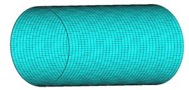
Fig. 5The response signals of three directions
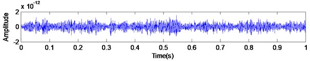
a) Response of direction about the 1118th observation spot
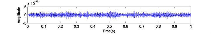
b) Response of direction about the 1118th observation spot
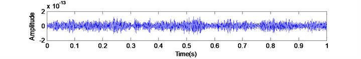
c) Response of direction about the 1118th observation spot
4.2. Evaluation criteria
In order to evaluate the effect of identification about the new method of three-dimensional structures, the mode shapes and natural frequencies are calculated by the finite element analysis (FEA) method as the real modal parameters to compare with the identified modal parameters. Modal assurance criterion (MAC) is an important criterion to reflect the effectiveness of the modal identification by the new method. The modal assurance criterion is defined as:
In Eq. (24), is a theoretical value by the FEA method of the th order mode shape and represents the identified value by the new method of th order mode shape. It is worth noting that the value of MAC ranges from 0 to 1, and the value closer to 1 states the higher accuracy of the identified mode shape.
4.3. Simulation verification results
From Fig. 5, the vibration response of the direction and the direction is larger than the direction, so according to Fig. 3 about the process of OMA for three-dimensional structures. At first the direction is decomposed by SOBI method. Then with the aid of the general reversion of least square algorithm, the other two directions are calculated. At last, identify the modal parameters of three-dimensional structure are identified by matrix assembly method. At the same time, another method is introduced to assemble three directions directly and then identify the modal parameters of three-dimensional structures directly is compared with the proposed method.
The modal vibration modes and natural frequencies by the FEA method are used as the real value, shown in Fig. 6.
Fig. 6Real mode shapes calculated by FEA
a) The 1th real modal shape
b) The 2th real modal shape
c) The 3th real modal shape
d) The 4th real modal shape
e) The 5th real modal shape
f) The 7th real modal shape
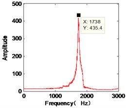
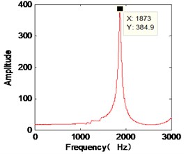
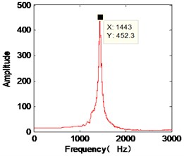
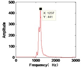
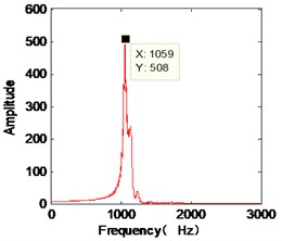
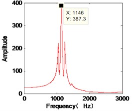
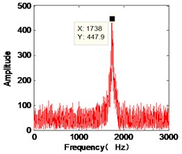
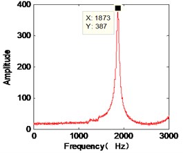
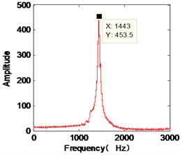
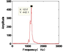
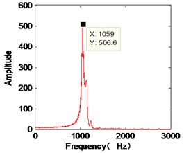
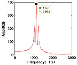
When the damping ratio of the cylindrical shell is 0.03, the mode frequency identified by the purposed algorithm is shown in Fig. 7. Table 1 and Table 2 are the identified frequency by the purposed algorithm comparison of the real frequency by FEA and the MAC of mode shapes respectively.
According to the identified modal shapes by the SOBI method, Table 3 shows the MAC values between each identified modal shape. Each modal shape of its self MAC value is 1, and one modal shape of MAC with other modal shapes are small and almost close to 0.
When the damping ratio of the cylindrical shell is 0.03 and with 5 % measurement noises, the mode frequency is identified by the purposed algorithm that is shown in Fig. 8 below. Table 4 and Table 5 are the identified frequency by the purposed algorithm comparison of real frequency by the FEA method and the MAC of mode shapes respectively.
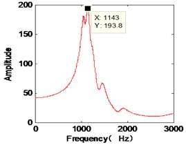
Fig. 7The identified mode frequencies when the damping ratio is 0.03
a) FFT of the 1th separated component
b) FFT of the 2th separated component
c) FFT of the 3th separated component
d) FFT of the 4th separated component
e) FFT of the 5th separated component
f) FFT of the 6th separated component
Table 1Comparison of natural frequencies with different methods
FEA method | The proposed method | Three directions assemble directly | |||||
Orders | Frequency (Hz) | Orders | Frequency (Hz) | relative error | Orders | Frequency (Hz) | Relative error |
1 | 1054.9 | 5 | 1059 | 0.389 % | 5 | 1059 | 0.389 % |
2 | 1145.7 | 6 | 1146 | 0.026 % | 6 | 1151 | 0.463 % |
3 | 1239.6 | 4 | 1237 | –0.210 % | 4 | 1237 | –0.210 % |
4 | 1441.9 | 3 | 1443 | 0.076 % | 3 | 1439 | –0.201 % |
5 | 1740.0 | 1 | 1738 | –0.115 % | 1 | 1738 | –0.115 % |
7 | 1871.7 | 2 | 1873 | 0.069 % | 2 | 1874 | 0.122 % |
Table 2MAC of modal shapes when the damping ratio is 0.03
FEA method | The proposed method | Three directions assemble directly | ||
Order of real modal shape | Order of identified modal shape | MAC | Order of identified modal shape | MAC |
1 | 5 | 0.8772 | 5 | 0.6532 |
2 | 6 | 0.6865 | 6 | 0.6179 |
3 | 4 | 0.5726 | 4 | 0.7937 |
4 | 3 | 0.5357 | 3 | 0.5365 |
5 | 1 | 0.5910 | 1 | 0.6220 |
7 | 2 | 0.9191 | 2 | 0.9194 |
Table 3MAC of modal shapes when the damping ratio is 0.03
Order | 1 (1059 Hz) | 2 (1146 Hz) | 3 (1237 Hz) | 4 (1443 Hz) | 5 (1738 Hz) | 7 (1873 Hz) |
1 (1059 Hz) | 1 | 0.0037 | 3.2338×10⁻⁴ | 2.1494×10⁻⁴ | 0.0894 | 5.4216×10⁻⁴ |
2 (1146 Hz) | 0.0037 | 1 | 0.0320 | 8.4117×10⁻⁴ | 1.9370×10⁻⁵ | 9.3939×10⁻⁴ |
3 (1237 Hz) | 3.2338×10⁻⁴ | 0.0320 | 1 | 1.2094×10⁻⁷ | 0.042 | 3.4047×10⁻⁵ |
4 (1443 Hz) | 2.1494×10⁻⁴ | 8.4117×10⁻⁴ | 1.2094×10⁻⁷ | 1 | 0.0479 | 8.0666×10⁻⁴ |
5 (1738 Hz) | 0.0894 | 1.9370×10⁻⁵ | 0.042 | 0.0479 | 1 | 0.0080 |
7 (1873 Hz) | 5.4216×10⁻⁴ | 9.3939×10⁻⁴ | 3.4047×10⁻⁵ | 8.0666×10⁻⁴ | 0.0080 | 1 |
Fig. 8The identified mode frequencies when the damping ratio is 0.03 and with 5 % measurement noises
a) FFT of the 1th separated component
b) FFT of the 2th separated component
c) FFT of the 3th separated component
d) FFT of the 4th separated component
e) FFT of the 5th separated component
f) FFT of the 6th separated component
Table 4Comparison of natural frequencies with different method with 5 % measurement noises
FEA method | The proposed method | Three directions assemble directly | |||||
Orders | Frequency (Hz) | Orders | Frequency (Hz) | Relative error | Orders | Frequency (Hz) | Relative error |
1 | 1054.9 | 5 | 1059 | 0.389 % | 5 | 1059 | 0.389 % |
2 | 1145.7 | 6 | 1146 | 0.026 % | 6 | 1147 | 0.113 % |
3 | 1239.6 | 4 | 1237 | –0.210 % | 4 | 1237 | –0.210 % |
4 | 1441.9 | 3 | 1443 | 0.076 % | 3 | 1443 | 0.076 % |
5 | 1740.0 | 1 | 1738 | –0.115 % | 1 | 1738 | –0.115 % |
7 | 1871.7 | 2 | 1873 | 0.069 % | 2 | 1873 | 0.069 % |
Table 5MAC of modal shapes when the damping ratio is 0.03 and with 5 % measurement noises
FEA method | The proposed method | Three directions assemble directly | ||
Order of modal shape | Order of identified modal shape | MAC | Order of identified modal shape | MAC |
1 | 5 | 0.5806 | 5 | 0.4938 |
2 | 6 | 0.4214 | 6 | 0.4113 |
3 | 4 | 0.4299 | 4 | 0.5184 |
4 | 3 | 0.3567 | 3 | 0.3572 |
5 | 1 | 0.2111 | 1 | 0.2741 |
7 | 2 | 0.6086 | 2 | 0.6102 |
When the damping ratio of the cylindrical shell is 0.03, Table 6 shows the mode shapes identified by finite element analysis, the purposed algorithm without noises and the purposed algorithm with 5 % measurement noises.
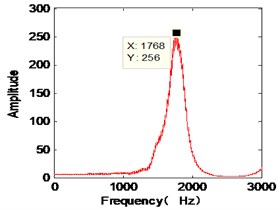
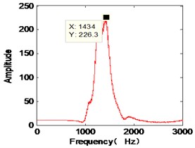
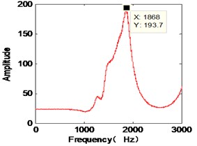
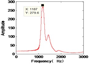
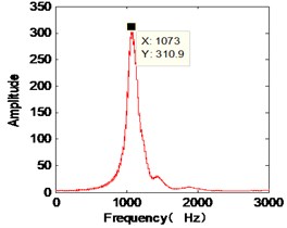
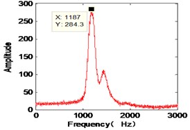
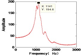
When the damping ratio of the cylindrical shell is 0.1, the mode frequency identified by the purposed algorithm is shown in Fig. 9. Table 7 and Table 8 is the identified frequency by the purposed algorithm comparison of real frequency by FEA and the MAC of mode shapes respectively. And “–” represents that the mode parameters are not identified.
Table 6Mode shapes when the damping ratio is 0.03
Method | Mode shapes | |||||
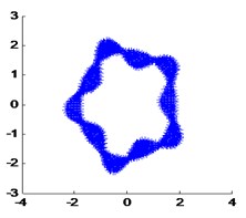
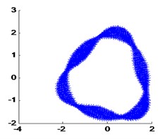
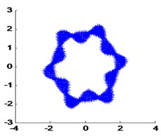
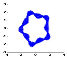
1th order | 2th order | 3th order | 4th order | 5th order | 7th order | |
FEA | 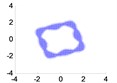 | 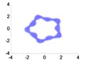 | 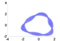 | 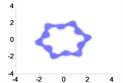 | 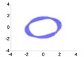 | 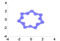 |
This method | 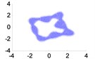 | 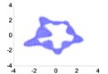 | 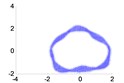 | 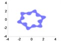 | 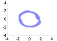 | 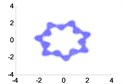 |
This method (5 % noise) | 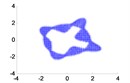 | 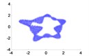 | 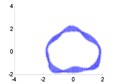 | 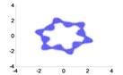 | 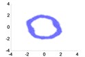 | 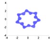 |
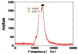
Fig. 9The identified mode frequencies when the damping ratio is 0.1
a) FFT of the 1th separated component
b) FFT of the 2th separated component
c) FFT of the 3th separated component
d) FFT of the 4th separated component
e) FFT of the 5th separated component
f) FFT of the 6th separated component
Table 7Comparison of natural frequencies with different method when the damping ratio is 0.1
FEA method | The proposed method | Three directions assemble directly | |||||
Orders | Frequency (Hz) | Orders | Frequency (Hz) | Relative error | Orders | Frequency (Hz) | Relative error |
1 | 1054.9 | 5 | 1073 | 1.716 % | 6 | 1044 | –1.033 % |
2 | 1145.7 | 6 | 1143 | –0.236 % | 4 | 1163 | 1.510 % |
3 | 1239.6 | 4 | 1187 | –0.424 % | – | -- | – |
4 | 1441.9 | 2 | 1434 | –0.548 % | 3 | 1434 | –0.548 % |
5 | 1740.0 | 1 | 1768 | 1.609 % | 1 | 1764 | 1.379 % |
7 | 1871.7 | 3 | 1868 | –0.198 % | 2 | 1868 | –0.198 % |
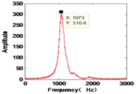
When the damping ratio of the cylindrical shell is 0.1 and with 5 % measurement noises, the mode frequency identified by the purposed algorithm is shown in Fig. 10. Table 9 and Table 10 are the identified frequency by the purposed algorithm comparison of real frequency by FEA and the MAC of mode shapes respectively.
Fig. 10The identified mode frequencies when the damping ratio is 0.1 with 5 % measurement noises
a) FFT of the 1th separated component
b) FFT of the 2th separated component
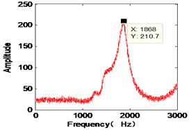
c) FFT of the 3th separated component
d) FFT of the 4th separated component
e) FFT of the 5th separated component
f) FFT of the 6th separated component
Table 8MAC of modal shapes when the damping ratio is 0.1
FEA method | The proposed method | Three directions assemble directly | ||
Order of modal shape | Order of identified modal shape | MAC | Order of identified modal shape | MAC |
1 | 5 | 0.7774 | 6 | 0.5255 |
2 | 6 | 0.4939 | 4 | 0.9204 |
3 | 4 | 0.3062 | – | – |
4 | – | – | 3 | 0.5108 |
5 | 1 | 0.0565 | 1 | 0.1407 |
7 | – | – | 2 | 0.9033 |
Table 9Comparison of natural frequencies with different method with 5 % measurement noises
FEA method | The proposed method | Three directions assemble directly | |||||
Orders | Frequency (Hz) | Orders | Frequency (Hz) | Relative error | Orders | Frequency (Hz) | Relative error |
1 | 1054.9 | 5 | 1073 | 1.716 % | 6 | 1044 | –1.033 % |
2 | 1145.7 | 6 | 1141 | –0.410 % | 4 | 1163 | 1.510 % |
3 | 1239.6 | 4 | 1187 | –4.243 % | – | – | – |
4 | 1441.9 | 2 | 1430 | –0.825 % | 2 | 1430 | –0.825 % |
5 | 1740.0 | – | – | – | 1 | 1752 | 0.690 % |
7 | 1871.7 | 3 | 1868 | –0.198 % | 3 | 1868 | –0.198 % |
Table 10MAC of modal shapes when the damping ratio is 0.1 with 5 % measurement noises
FEA method | The proposed method | Three directions assemble directly | ||
Order of real modal shape | Order of identified modal shape | MAC | Order of identified modal shape | MAC |
1 | 5 | 0.5175 | 6 | 0.4096 |
2 | 6 | 0.2984 | 4 | 0.6367 |
3 | 4 | 0.2364 | – | – |
4 | – | – | 2 | 0.3448 |
5 | – | – | – | – |
7 | – | – | 3 | 0.6120 |
When the damping ratio of the cylindrical shell is 0.1, Table 11 shows the mode shapes identified by finite element method, the purposed algorithm without noises and the purposed algorithm with 5 % measurement noises.
Table 11mode shapes when the damping ratio is 0.1
Method | Mode shapes | |||||
1th order | 2th order | 3th order | 4th order | 5th order | 7th order | |
FEA | 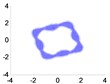 | 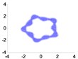 | 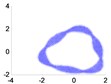 | 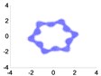 | 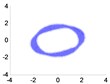 | 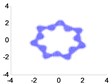 |
This method | 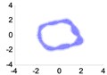 | 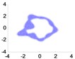 | 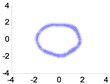 | 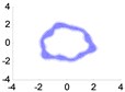 | – | 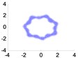 |
This method (5 % noise) | 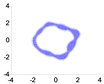 | 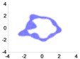 |  | – | – | – |
4.4. Results analysis
1) From the result identified by the purposed method, Fig. 7 and Fig. 9 show the identified modal frequencies with different damping ratios, by comparing with the frequencies calculated by the FEA method in Table 1 and Table 7. The modal frequencies identification precision changes when damping ratios increases. However, the relative errors are under 5 %. Table 6 and Table 11 show the mode shapes under different methods.
2) From Table 1, Table 4, Table 7 and Table 9, the order of identified modal frequencies and real modal frequencies are not one-to-one correspondence. The reason is that the order of the mode coordinate vector is uncertainty according to Eq. (14).
3) From all the results, the 6th order modal parameters are not identified because of its small modal contribution in dynamic response measurement signals.
4) With the increasing of damping ratio, the identified mode shapes are becoming deformed. It is more difficult to identify the modal parameters because the larger of damping ratio, the smaller of response of the structure.
5) Contrasting Fig. 7 with Fig. 8, and from Table 4 and Table 9. In conclusion, this method is robustness to Gauss measurement noises disturbances. Because second order statistics rather than higher-order statistics method is used in SOBI method.
5. Conclusions
In this paper, we proposed an OMA method about SOBI of three-dimensional structures. This new method takes advantages of the SOBI algorithm and the general reversion of least square algorithm to identify the modal parameters of three-dimensional structures. Modal parameters of three-dimensional structures are more difficult than that of one-dimensional, especially in mode shape.
With the increasing of modal damping, the mode shape of structures will gradually into the complex mode field with the increasing error of three directions. How to identify the vibration response in small contribution model and keep the better identified results when damping ratios increases needs more researches in the future.
References
-
Rainieri C., Fabbrocino G. Operational Modal Analysis of Civil Engineering Structures: an Introduction and Guide for Applications. Springer, 2014.
-
Huajun L., Hezhen Y. Research progress on modal parameter identification and damage diagnosis for offshore platform structures. Engineering Mechanics, Vol. 21, Issue 1, 2004, p. 116-138.
-
Devriendt C., Magalhães F., Weijtjens W., et al. Structural health monitoring of offshore wind turbines using automated operational modal analysis. Structural Health Monitoring, Vol. 13, Issue 6, 2014, p. 644-659.
-
Reynders E., Houbrechts J., De Roeck G. Fully automated (operational) modal analysis. Mechanical Systems and Signal Processing, Vol. 29, 2012, p. 228-250.
-
Rizzo A. A., Giannoccaro N. I., Messina A. Analysis of operational modal identification techniques performances and their applicability for damage detection. Key Engineering Materials, Trans Tech Publications, Vol. 628, 2014, p. 143-149.
-
Reynders E. System identification methods for (operational) modal analysis: review and comparison. Archives of Computational Methods in Engineering, Vol. 19, Issue 1, 2012, p. 51-124.
-
Poncelet F., Kerschen G., Golinval J. C., et al. Output-only modal analysis using blind source separation techniques. Mechanical Systems and Signal Processing, Vol. 21, Issue 6, 2007, p. 2335-2358.
-
Zhou W., Chelidze D. Blind source separation based vibration mode identification. Mechanical Systems and Signal Processing, Vol. 21, Issue 8, 2007, p. 3072-3087.
-
Kerschen G., Poncelet F., Golinval J. C. Physical interpretation of independent component analysis in structural dynamics. Mechanical Systems and Signal Processing, Vol. 21, Issue 4, 2007, p. 1561-1575.
-
Belouchrani A., Abed-Meraim K., Cardoso J. F., et al. A blind source separation technique using second-order statistics. IEEE Transactions on Signal Processing, Vol. 45, Issue 2, 1997, p. 434-444.
-
Toumi I., Caldarelli S., Torrésani B. A review of blind source separation in NMR spectroscopy. Progress in Nuclear Magnetic Resonance Spectroscopy, Vol. 81, 2014, p. 37-64.
-
Antoni J., Chauhan S. A study and extension of second-order blind source separation to operational modal analysis. Journal of Sound and Vibration, Vol. 332, Issue 4, 2013, p. 1079-1106.
-
Rainieri C. Perspectives of second-order blind identification for operational modal analysis of civil structures. Shock and Vibration, Vol. 2014, 2014.
-
Poncelet F., Kerschen G., Golinval J. C., et al. Second-order blind identification for operational modal analysis. ASME International Design Engineering Technical Conferences and Computers and Information in Engineering Conference. American Society of Mechanical Engineers, 2007, p. 439-445.
-
Wang C., Guan W., Gou J., et al. Principal component analysis based three-dimensional operational modal analysis. International Journal of Applied Electromagnetics and Mechanics, Vol. 45, Issues 1-4, 2014, p. 137-144.
-
Handbook of Blind Source Separation: Independent Component Analysis and Applications. Academic Press, 2010.
-
Wang C., Gou J., Bai J., et al. Modal parameter identification with principal component analysis. Journal of Xi’an Jiaotong University, Vol. 47, Issue 11, 2013, p. 97-104.
-
Basov K. A. ANSYS and LMS Virtual Lab. Geometric Modeling, 2006, p. 240.
-
Zhang X. Matrix Analysis and Applications. Tsinghua and Springer Publishing House, Beijing, 2004, p. 71-100.
-
Wang C., Lai X., Jiao J., et al. Load identification of acoustic and vibration sources following linear regression and least-squares of generalized matrix inverse method. Journal of Information and Computational Science, Vol. 11, Issue 9, 2014, p. 3229-3239.
Cited by
About this article

This work was financially supported by National Natural Science Foundation of China (Grant No. 51305142), Science and Technology Program Guiding Project of Fujian Province (Grant No. 2017H01010065), the General Financial Grant from the China Postdoctoral Science Foundation (Grant No. 2014M552429), Postgraduate Scientific Research Innovation Ability Training Plan Funding Projects of Huaqiao University (Grant No. 1400214012).
