Abstract
This paper presents a strategy for computational modelling of elastic rubber couplings under dynamic loading. Methods how to determine static and dynamic characteristics of the elastic coupling based on static and dynamic experimental tests of rubber elements are presented. The nonlinear deformation behaviour, frequency and temperature dependent properties of rubber are considered for computational models. The model is applied to the elastic coupling connecting an in-line six-cylinder natural gas engine and an electrical generator. Loading forces are based on in-cylinder pressure measurement. Experimental verification of the computational model results is carried out by measuring the values on a test engine using the non-contact laser measuring technique.
1. Introduction
Modern powertrains that are based on internal combustion engines (ICE), are developed as highly efficient systems which transfer primary energy source, like diesel or compressed natural gas, to output energy like vehicle kinetic energy, electricity or heat. Powertrains often contain elastic components to reduce vibrations. Such components are often made of rubber – e.g. rubber torsional dampers, rubber couplings or engine mounts. These components are often highly thermally, mechanically and chemically stressed and require special procedures when designing them.
In general, rubber materials are used to reduce vibrations of machines. However, to correctly predict the vibration response of a machine, the dynamic properties of rubber components, such as the Young’s modulus or the damping factor, have to be accurately identified.
Many authors present computational and experimental approaches of how to model rubber components. Some of them have carried out an experimental research by directly measuring the Young’s modulus and the damping factor. Sim et al. [1], for example, developed a technique to calculate the rubber material properties of viscoelastic materials with finite element method (FEM). They derived the Young’s modulus, the damping factor and the Poisson’s ratio from two different rubbers with various shape factors. Koblar et al. [2] presented a similar method for describing the dynamic behaviour of rubber components. Lin et al. [3] developed a method to evaluate the frequency-dependent stiffness and damping properties of rubber mounts by using the measured response function from the impact test. Rubber dynamic behaviour is also discussed in detail by Sjöberg [4] and Olsson [5].
Vibrational problems of powertrains are commonly solved by using a wide range of experimental or computational approaches. Experimental methods are often very expensive; and therefore, rapid developments of modern computational methods with highly specialized computational models are in demand.
Present state-of-the-art in powertrain vibration simulations consists of computational models solved in time domain using Multibody systems (MBS) with high share of flexible bodies, often based on FEM principles. Some powertrain components, e.g. flywheels or pulleys, are included only as an additional mass, or frequently, they are not included at all. Crankshaft and engine block interactions are often solved by using a hydrodynamic, or more advanced elastohydrodynamic model of a slide bearing. However, full elastohydrodynamic solution of Reynolds equation, including shell and pin deformations, is still not fully adopted for powertrain dynamics with many slide bearings. Examples of computational approaches verified by measurement are presented in Novotny [6, 7] or Offner [8].
2. Objectives of the computational modelling
The main objective is to develop a complex methodology to predict the dynamic properties of elastic couplings based on a component testing of rubber elements. The resulting computational tool has to have following properties:
• Non-linear deformation, frequency and temperature dependent behavior of rubber elements.
• Ability to assemble the elastic couplings into large powertrain models.
• Inputs based on results of static and dynamic component tests of the rubber element.
3. Modelling of properties of elastic coupling
3.1. Experimental determination of static properties of rubber element
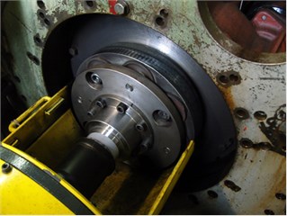
To determine the characteristics of the entire coupling in a given configuration requires analysis of static properties of a single rubber element in dependence on deformation, temperature and frequency. The design of the current coupling includes eight individual rubber elements embedded into the steel disc, see Fig. 1. These elements allow the formation of various configurations of couplings with defined properties.
Fig. 1Elastic coupling connecting engine and electric generator
The nonlinear behavior of the rubber elements of the coupling has to be included in the model. Rubber element nonlinearities, due to amplitude dependence, are discussed by Harris and Stevenson [9]. These impacts can be caused by the geometrical design of the rubber component, as well as, by the intrinsic material behavior. The references present nonlinear stress of the material – strain relations for finite strain ranging approximately from 20 to 500 %. Components also show nonlinear properties for small to intermediate amplitudes – ranging approximately up to 5 % of component strain due to the material behavior.
Rubber element properties are analyzed separately by technical experiments and computational models. Subsequently, the whole coupling properties are derived. Static deformation properties of rubber element assume the following:
• Deformation in the radial direction (corresponding to the load of the element perpendicular to the axis of the element).
• Deformation in the axial direction (corresponding to the load of the element in the axis of the element).
• Angular deformation perpendicular to the axis of the element (corresponding to the moment perpendicular to the axis of the element).
A determination of these components is carried out employing experimental procedure for computational model calibrations and using computational procedure for radial, axial and angular directions. The results of the radial loading are based on basic technical experiments which are used to tune computational finite element (FE) model properties.
The static characteristics of the rubber element are determined by using the universal testing machine, see Fig. 2.
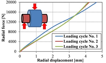
The radial loading characteristics of the rubber element is presented in Fig. 3. It shows three repetitions of loading, the first cycle is slightly different due to element positioning, therefore this case is not assessed.
Fig. 2Arrangement of a technical experiment to determine the static characteristics of the rubber element
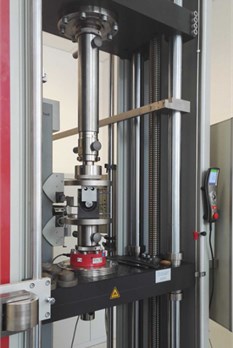
Fig. 3Measured force vs. radial deformation
3.2. Computational determination of static properties of rubber element
It is not possible to measure all the necessary elastic properties of a rubber element. However, there is a way how to obtain all the properties to use computational determinations of static properties of rubber elements based on the selected experimental results. The experimental results are used to tune the computational model of the rubber element. The computational model is solved by entering the displacement in a given direction and by evaluation of the overall force required for implementation of the displacement.
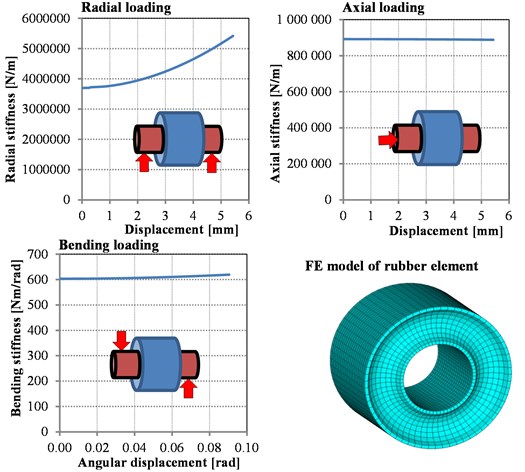
The computational determination of the deformation properties of the rubber element is performed using the finite element method (FEM). Mooney-Rivlin’s two-parameter hyperelastic model is used as rubber material model. The Mooney-Rivlin’s parameters taken from measured results presented in Fig. 3. The resultant material constants characterizing the deformation of the deviatoric stress are 1.11 and 0.27 and incompressibility parameter is 0.018.
The calculation results, including the introduction of the FE model, are presented in Fig. 4.
Fig. 4Calculated radial, axial and bending stiffness of single rubber element and FE mesh of computational model
Nonlinear deformation behavior of the rubber element is considered only in the radial direction and it can be approximated as:
where is radial stiffness for current radial loading, is radial stiffness for no loaded state and radial deformation of the rubber element center under current loading. Current radial stiffness can be evaluated as:
where is a current radial force.
Axial stiffness and bending stiffness of the rubber element are considered as constant with respect to the values of the axial forces or bending moments. The nonlinear deformation behavior is not presumed.
3.3. Experimental determination of dynamic characteristics of rubber element
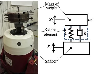
Material components made of rubber present a significant dependence on the loading frequency. These frequency dependent properties are determined experimentally by a vibration exciter device. The assembly of the technical experiment to determine the dynamic characteristics of rubber element, is presented in Fig. 5.
The technical experiment is carried out in above-resonance area of the system consisting of the rubber element and a weight. The following parameters are evaluated:
radial dynamic stiffness of rubber element and relative damping of rubber.
The description of the experimental arrangement used for measurement can be simplified to a system with one degree of freedom. Therefore, the equation of the motion, of a system presuming only harmonic loading, is:
where is a defined time dependent displacement of the vibration excitation, is a response of weight mass , is radial viscous damping coefficient of a rubber element, is radial stiffness of a rubber element, is angular velocity and is time.
Fig. 5Arrangement of technical experiment to determine the dynamic characteristics of the rubber element
The system can be solved by introducing complex variables. Then the complex dynamic stiffness of the rubber element is defined as:
The quantities with vinculum are complex; therefore, the rubber element radial stiffness can be calculated as:
And radial damping coefficient of the rubber element is:
Relative damping is believed to be independent of the excitation frequency:
Measuring and evaluating the radial stiffness and the relative damping is performed with the excitation frequency ranging from 50 Hz to 300 Hz and for temperatures from 25 °C to 55 °C. The measured stiffness dependent on excitation frequency, is expressed in the form of frequency correction coefficients. These correction coefficients are defined as:
where is a frequency correction coefficient for stiffness and is a frequency correction coefficient for relative damping. The measured frequency correction coefficient for stiffness is presented in Fig. 6.
The measured frequency correction coefficient for stiffness can be approximated by second order polynomial as:
And measured frequency correction coefficient for relative damping is a constant equal to 1.
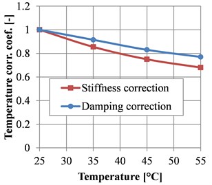
The influence of temperature can be expressed by temperature correction coefficient for stiffness and relative damping The measured values of temperature correction coefficients are presented in Fig. 7.
The values of the temperature correction coefficients for stiffness and relative damping can be expressed by second order polynomial as:
Fig. 6Measured frequency correction coefficient for stiffness
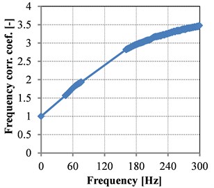
Fig. 7Measured temperature correction coefficient for stiffness and relative damping
3.4. Determination of dynamic nonlinear characteristics of elastic coupling
The resultant static torsional stiffness of the whole elastic coupling can be calculated as follows:
where is a pitch diameter of rubber elements, is a number of rubber elements on one side and is a total number of rubber elements.
The resulting dependency of coupling dynamic stiffness on the loading frequency and element temperature can be written as:
where is static coupling stiffness at temperature of 25 °C and under static load. Relation of viscous damping coefficient , relative damping and frequency is:
Relative damping dependent on temperature can be expressed as:
where is relative damping at temperature of 25 °C. It is supposed that the dependence of relative damping on the loading frequency is minimal; and therefore, the frequency dependence is not included in the relative damping Eq. (15).
The coupling model is extended by coupling flexibility for load in axial direction and for bending moments. These properties are considered as independent of the deformation. The bending stiffness of the whole coupling can be approximated as:
And coupling bending damping reads:
Similarly, the axial stiffness of the whole coupling is defined as:
And the axial damping can be calculated as:
where is axial deformation velocity.
4. Application of elastic coupling on connection of engine and generator
The developed approach is a general procedure used for modelling rubber components of powertrains, such as couplings, dampers or engine mounts. The modelling abilities and verification of computational results are presented on the elastic coupling connecting ICE and electric generator. The target engine is a turbocharged six-cylinder engine using compressed natural gas (CNG) as fuel. The main engine parameters are: engine displacement of 11.9 liters and peak power output of 250 kW at engine speed of 1 800 rpm. Idling speed of the engine is 800 rpm.
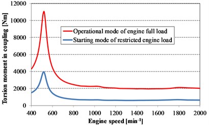
There are two operational modes of this engine:
• Operating mode considering full engine load for engine speed 1000-2000 rpm.
• Starting mode considering restricted engine load for engine speed 400-1000 rpm.
Engine speeds below the engine idling speed of the engine do not occur in engine operation, but they are presented to demonstrate the properties of the elastic coupling.
The model for a solution of ICE and electric generator system vibrations, is based on multibody system and comprises of two subsystems:
• Virtual crank train including all the significant components of crank train.
• Computational model of elastic coupling including deformation, frequency and temperature dependencies.
The model is assembled, as well as, numerically solved in multibody system ADAMS. ADAMS is a general code and enables the integration of user-defined models directly using ADAMS commands or using user written FORTRAN or C++ subroutines. ADAMS C++ solver of version 15 is used for numerical calculation of the results.
4.1. Implementation of computational models
The computational model is solved in time domain for steady state conditions. Model of crank train and generator system, including the elastic coupling assembled in multibody system, is shown in Fig. 8. Full description of crank train computational models are presented in Novotny [6].
The computational model of the elastic coupling comprises of two bodies (discs) connected by nonlinear general forces enabling flexibility for torsional, bending and axial loading. The two coupling bodies are constrained by primitive joint enabling one axial translational movement and three rotational movements. The computational model of crank train is excited by gas forces in combustion chambers considering operational states of the ICE.
The computations of the engine-generator system are done for steady states starting from engine speed 400 rpm to engine speed 2000 rpm with step of 100 rpm.
The computed results presented in Fig. 9 show torsional resonance of the 3rd order near the engine speed 520 rpm, this engine speed is highly critical; however, the resonance occurs below engine operating speed range.
Operating speeds show no torsional resonances of the engine-generator system. In general, a lack of resonances near the operating engine speeds is critical in terms of the coupling design.
Fig. 8Model of crank train and generator system including elastic coupling assembled in multibody system
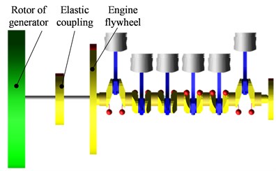
Fig. 9Computed torsional moments in the elastic coupling for engine speeds including starting and operational engine modes
4.2. Experimental verification of computational models
Technical experiments (see Fig. 10) are proposed to verify the final design of the elastic coupling, as well as, to validate computational models. The verification of the coupling design is performed in the engine operating speed range under full engine load conditions. Resonant speed of the engine-generator system cannot be directly verified because in such low speeds, below idling speed, the engine does not operate.
Fig. 10Measurement of crankshaft pulley angular vibrations
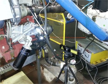
Fig. 11Dominant harmonic orders vs. engine speed for computed (“Comp.”) and measured (“Exp.”) angular displacements
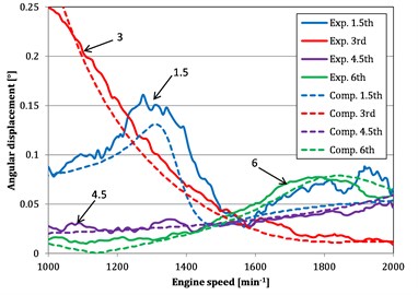
Dominant harmonic orders vs. engine speed for computed and measured angular displacements of flywheel pulley are presented in Fig. 11. The 3rd harmonic order is closely connected with vibration of ICE and the electric generator system. The coupling is always designed to avoid resonances in operational engine speeds.
5. Conclusions
The proposed methodology uses a combination of various experimental and computational approaches to determine the rubber coupling parameters based on simple component tests involving the determination of load, temperature and frequency properties of the rubber component.
Using this methodology, it is possible to avoid problems with high thermomechanical loads of coupling components at the design phase. Moreover, the methodology based on testing the component of the clutch enables the configuration parameters of different connectors and thus to effectively build a coupling for lower or higher loads.
Methodology and the elastic coupling is also verified in the case of the connection of the ICE and generator in real environment. The torsional resonance of the 3rd order is distant from the operating speed range and the coupling design is confirmed, as well as, computational models of the coupling. Measurement results of torsional vibrations confirmed the accuracy of the methodology used for that purpose.
However, there are some problematic areas that cannot be described with high accuracy. These include inconsiderable variability in the properties of rubber or external conditions during operations of the engine-generator system.
References
-
Sim S., Kim K. J. A method to determine the complex modulus and Poisson’s ratio of viscoelastic materials from fem applications. Journal of Sound and Vibration Vol. 141, Issue 1, 1990, p. 71-82.
-
Koblar D., Bolteza M. Evaluation of the frequency-dependent Young’s modulus and damping factor of rubber from experiment and their implementation in a finite-element analysis. Experimental Techniques, 2013, https://doi.org/10.1111/ext.12066.
-
Lin T. R., Farag N. H., Pan J. Evaluation of frequency dependent rubber mount stiffness and damping by impact test. Applied Accoustics, Vol. 66, 2005, p. 829-844.
-
Sjöberg M. On Dynamic Properties of Rubber Isolators. Doctoral Thesis, Royal Institute of Technology, Stockholm, 2002.
-
Olsson K. A. Finite Element Procedures in Modelling the Dynamic Properties of Rubber. Doctoral Thesis, Lund University, Lund, 2007.
-
Novotny P. Virtual Engine – A Tool for Powertrain Development. Habilitation Thesis, Brno University of Technology, Brno, 2009.
-
Novotný P., Prokop A., Zubík M., Řehák K. Investigating the influence of computational model complexity on noise and vibration modeling of powertrain. Journal of Vibroengineering, Vol. 18, Issue 1, 2016, p. 378-393.
-
Offner G., Priebsch H. H., Krasser J., Laback O. Simulation of multi-body dynamics and elastohydrodynamic excitation in engines in special consideration of piston-liner contact. Journal of Multi-body Dynamics, Part K, 2001.
-
Harris J., Stevenson A. On the role of nonlinearity in the dynamic behavior of rubber components. Rubber Chemistry and Technology, Vol. 59, Issue 5, 1986, p. 740-764.
About this article

The research leading to these results has received funding from the Ministry of Education, Youth and Sports under the National Sustainability Programme I., Project No. LO1202. The authors gratefully acknowledge this support.
