Abstract
This paper presents results of numerical analysis for the seismic response of hydropower station intake tower in step-like ground based on artificial boundary theory. A L topography finite element model was established to verify the correctness of the proposed method of viscous elasticity boundary by consider inconsistent reflective surface. The method was applied to an intake tower, and the acceleration of bedrock was obtained by seismic inversion method, then the equivalent load of each node was calculated. Five different models were established as follow: massless foundation, consistent input viscous elasticity boundary, inconsistent input viscous elasticity boundary and whether set contact, then displacement and stress were compared, the results show that the proposed method with contact was minimal. The base plate of intake tower and the foundation were in close adhesion state in the whole process of earthquake, both sides and rear side of intake tower without through disengagement phenomena from rock, it can conclude that the intake tower in the overall stability state.
1. Introduction
Intake tower is an accessory and has less research concerns than the major in hydropower station, as the project throat it plays an important role in the seismic safety of water control project [1]. Bank-tower intake is a commonly used form of inlet that usually set in L-shaped rock terrain. Although its stability is better than the isolated inlet, the connection form between the intake tower and the mountain that has great influence on the deformation and stress of inlet.
The seismic parameters and the way of loading are important to the results of engineering seismic analysis. When the ground acceleration is known, the seismic data of the bedrock can be obtained by the inversion method [2], which makes the seismic load more reasonable.
In dynamic analysis, a certain range of foundation is usually intercepted, so as to consider the influence of elastic foundation on the superstructure [3-7]. The influence of radiation damping of foundation must be considered in a limited range of foundation. Local artificial boundary can be partial decoupling in time and space, and has good stability, efficiency and practicality in universal application [8]. As a local artificial boundary, many scholars [9] had made a detailed study of the viscoelastic boundary, the results show that it has high precision and stability, also easy to be implemented in the finite element software.
Scholars [10, 11] used the three-dimensional viscoelastic artificial boundary on the intake tower in dynamic analysis proved the method gets a good accuracy and applicability. Three-dimensional viscoelastic boundary derived base on assuming the spherical boundary [12]. The ground should be flat, no larger fluctuation and mutation. However, in the project the bank-tower intake with high surrounding rock, the tower is in a steep topography.
Zhao et al. [13, 14] study on the viscoelastic boundary of basin topography, the seismic wave motion of stepped topography is solved by using the technique of virtual symmetric substructure, and research shows that free face displacement amplitudes increase and the gradient of slope increases the dynamic amplification effect is more obvious. These studies used symmetrical or virtual processed the high and low side into 2D equally high boundary to avoid the viscoelastic boundary inconsistent input problem for the steep topography. But the back-tower intake location at 3D L-shape topography, before and after the tower, there is a high-level of mutation not a gradient slope, and dynamic analysis needs three direction seismic input, so it cannot transform into two-dimensional problems. Therefore, these methods cannot solve the problem completely. The connection between the tower and the backfill concrete and the rock is not completely consolidated, and different height or form of backfill concrete has a significant impact on the intake tower [15, 16]. Li et al. [17, 18] analyses the model of set contact between the intake tower and the surrounding rock, results show the tensile stress of tower can be released and the stress level reduced; these results close to the actual condition. However, these studies are based on the massless foundation without considering the effect of the foundation radiation damping.
This paper presents a method to realize the viscoelastic boundary of the intake tower with high surrounding rock. A numerical experiment is given to verify the correctness of the proposed method. Five finite element models with different boundary conditions are calculated, and the results are discussed. Finally, some suggestions are put forward for engineering practice.
2. Calculation theory and method validation
2.1. Viscoelastic artificial boundary theory
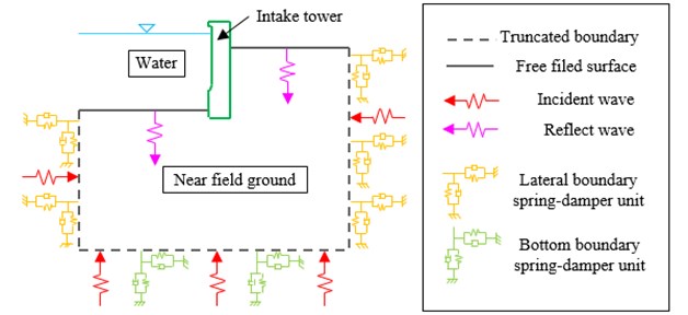
Viscoelastic artificial boundary absorbs the energy of scattered waves which spread from the upper by adding spring-damper unit on truncated boundary node, at the same time it reflects the resilience of the elastic medium. The acceleration and displacement are transformed into the equivalent nodal force on the artificial boundary; its Eq. (1) is:
where denote the equivalent nodal forces acting on the artificial boundary node, , are the stiffness matrix and the damping matrix, and , are the free field displacement and velocity vectors.
The node damping coefficient and the spring stiffness coefficient of viscoelastic artificial boundary can be calculated as follows [19]:
Normal boundary:
Tangential boundary:
where , is denote the density and the shear modulus of the medium; and are the propagation velocity of shear wave and compression wave in the medium. is the distance from the artificial boundary node to the scattering source; and are the normal and tangential stiffness correction coefficient.
2.2. The frequency domain inversion of seismic for bedrock motion
The seismic acceleration of bedrock is different from that of the free field [20]. As known ground acceleration time history, the seismic acceleration can be obtained from the frequency-domain inversion.
In the layered field, the inversion of the ground motion time history to the bedrock is carried out based on the theory of transient seismic response of linear hysteresis layer. The process is generally as follows: After read, the earthquake acceleration transform the transient waves into steady wave by using Dispersed Fourier Transform, the Fourier spectra of the composite is obtained by calculating the steady wave of the deep strata, by using the inverse Fourier Transform the time history of ground motion then obtained [21].
2.3. Type L terrain seismic input
The height of the free field surface of pre-and post the bank-tower intake composites a L-shape topography, the same height of the free surface seismic motion input was unreasonable [22-24]. The viscoelastic boundary should be study deeply for this situation.
First, a numerical experiment is made to validate the viscoelastic artificial boundary program. Some principles of displacement time history curves are getting to infer whether the proposed method is correct.
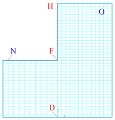
Two finite-element models were established (Fig. 1). Model A size: 100 m×100 m×50 m (length, width, height); model B size: 100 m×100 m×100 m (length, width, height). Spring-damper units were set at the bottom face and the four sides, then three directions stiffness coefficient and damping coefficient were calculated to complete the viscoelastic artificial boundary. Consider the wave propagation effects, the displacement and velocity time history of each node were generated by program, then the equivalent load on the node can be computed.
Fig. 1The 50 m and 100 m height finite element model and monitoring points
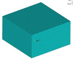
a) Model A
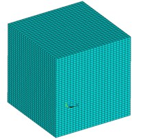
b) Model B
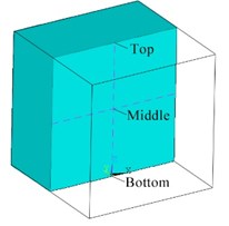
c) Schematic diagram of monitoring points
Material parameters, velocity and displacement inputs are referred in literature [25]. Material properties are defined as follows: elastic modulus = 24 MPa, Poisson’s ratio = 0.2 and density = 1000 kg/m3.So, shear wave velocity 100 m/s, shear modulus 10 MPa, compression wave velocity 163.3 m/s. The material damping coefficient is zero, and the expressions of displacement and velocity function are as follows:
In order to observe the displacement of every moment setting up three monitoring points at the bottom, middle and top of the model’s center line as shown in Fig. 1. The input wave transmitted in sequence at different depth points in the medium, when the peak value of the displacement wave spreads to the ground surface, the value of incident and reflected waves were superposed, the maximum displacement value is two times the peak value of the incident wave.
The displacement time history curve at three monitoring points Fig. 1(c) of models are shown in Fig. 2. From the figure, the peak value and the propagation curve shape of the wave obtained by numeric solution Fig. 2(b) and Fig. 2(d) are close to the theoretical solution Fig. 2(a) and Fig. 2(c), which proves the correctness of the viscoelastic artificial boundary program.
Establish a typical L-shape model, its size as shown in Fig. 3(a), and the location of each monitoring point marked in the intermediate profile as shown in Fig. 3(b). Part the vertical stepped terrain model into pre-and post-two parts as shown in Fig. 4, equivalent load time history of each layer was calculated that the pre-and post of upper free surface as the reflection face.
Fig. 2The horizontal displacement of monitoring points
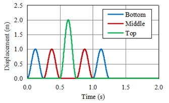
a) Theoretical solution of horizontal displacement of monitoring points in model A
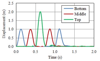
b) Numerical solution of horizontal displacement of monitoring points in model A
c) Theoretical solution of horizontal displacement of monitoring points in model B
d) Numerical solution of horizontal displacement of monitoring points for model B
Fig. 3L-shape finite element model and monitor points
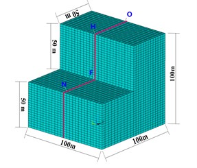
a) The diagram of 3D finite-element model size and observation point
b) The diagram of intermediate profile of model and monitoring points
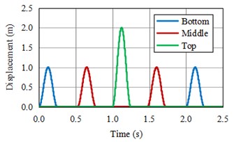
The horizontal displacement of the monitor points N and O of L-shape model as shown in Fig. 5(a). These two points are close to the left and right sides, the peak value of two monitor points’ displacement about 2 meters, its consistent with the theoretical value and all appear in the moment of conformity with the theoretical time (With the reference to Fig. 2(a) and Fig. 2(c), respectively), it presents that the loading method of viscoelastic artificial boundary for step topography is feasible. At the same time, from the displacement curve, it shows that the points N and O still have positive or negative displacement after the wave propagation over at about 1.25 s, these are different from the situation of model A or B, it can be inferred that wave will engender unbalanced force to result displacement when wave propagate in the medium with height difference.
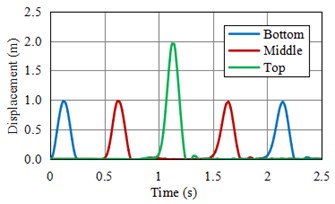
The horizontal displacement curve of three nodes from bottom to top at the height mutation position of model midplane are shown in Fig. 5(b), the curve shape and peak value of these three nodes’ displacement time history are totally different from model A or B, the peak value of monitor point H at the surface top appears a little later than the point O at the same height , and the value larger than the superposition value 2 meters of incident and reflection, this shows the volley face has a special amplification effect, and there has a larger negative displacement before the wave propagates to the point H; The peak displacement value of point F less than the point N’s value 2 meters, but greater than input displacement peak value 1 meter, and half the value of point H. This is due to the model before and after the application of the load imbalance has produced additional torque. The peak value of each monitor point has good proof to literature [8]. It shows reasonable methodology.
Fig. 4The calculate partition plan of vertical step model
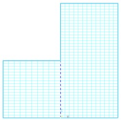
Fig. 5Numerical solution of displacement time history of observation point of step model
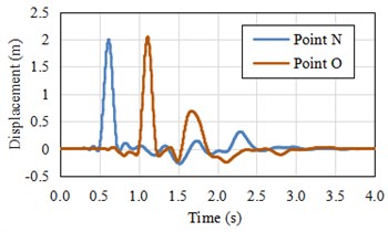
a) The horizontal displacements of point N and O on model free face
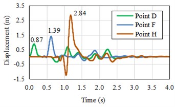
b) The horizontal displacements of the nodes from bottom to top at the middle line of model
Based on analysis and verification above, establishment the viscoelastic artificial boundaries system of the intake tower is shown in Fig. 6.
Fig. 6The schematic diagram of viscous artificial boundary system of intake tower
3. Model and loads
3.1. The basic parameters of intake tower
Based on the spillway tunnel intake tower of a real hydropower project, the elevation of base plate of the intake tower is 1635.00 m, the thickness of bottom plate is 5.0 m, the top elevation of inlet is 1716.00 m, and height of the inlet is 86 m. The normal water level is 1710.00 m. There are 35 meters backfill beside and behind the tower and connect with surrounding mountain. The level for seismic design of water release structure is exceeding probability of 5 % in 50 years; the peak motion acceleration value is 201.0 gal. The corresponding seismic fortification intensity is VIII. Engineering material parameters are provided in Table 1 and Table 2.
Table 1Mechanical parameters of concrete
Concrete grade | Static axial compressive strength (MPa) | Static elastic modulus (MPa) | Poisson ratio |
C30 | 26.2 | 3.00×10⁴ | 0.167 |
Table 2Tower foundation rock mechanical parameters
Rock mass classification | Dry density / cm3 | Compressive strength | Modulus | Shear strength | |||
Dry | Saturated | Elastic modulus | Deformation modulus | Concrete / rock | |||
MPa | GPa | (MPa) | |||||
III | 2.70 | 60 | 40 | 10 | 8 | 0.8 | 0.7 |
3.2. The finite element model and load condition
The model with finite-element software and use space Cartesian coordinate system, setting the coordinates origin in the center of the front side of inlet height of base plate of the intake tower, the axis pointing along the direction of flow; the axis is perpendicular to the direction of flow; the axis along the height direction of the tower. The depth of foundation is one time the height of the tower, the upstream and downstream foundation size is 50 m, the left and right sides are the same. Three-dimensional solid element is adopted for the tower and the foundation rock, and the inertia effect of the water on the tower is reflected by the addition mass element [1].
Tower-foundation finite element model as shown in Fig. 7.
There are five cases calculated to compare which listed in Table 3.
Fig. 7The tower-foundation finite element model
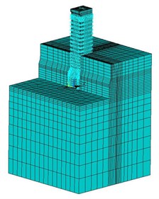
a) The whole model
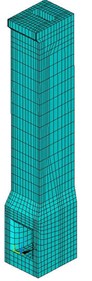
b) The intake tower
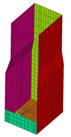
c) The contact element area
For model 2 and 4, the flexible-to-flexible body surface-to-surface 3D contact element are set between the tower and the surrounding mountain so that can simulate the state like crack or slip or contact between tower and rock during an earthquake Fig. 7(c). For face-to-face contact element, the improved Lagrange algorithm was used.
The seismic response spectrum given by the geological survey as the target spectrum to generate horizontal and vertical acceleration of earthquake wave, the fitting response spectrum and the target spectrum error are less than 5 %, and the acceleration baseline correction is carried out.
Table 3Model cases
Model name | Model condition description |
Model 1 | Massless foundation, not consider contact |
Model 2 | Massless foundation, consider contact |
Model 3 | Viscoelastic boundary considering the terrain, the contact is not considered |
Model 4 | Viscoelastic boundary considering the terrain, the contact is considered |
Model 5 | Viscoelastic boundary not considering the terrain, the contact is not considered |
Fig. 8The artificial fitted acceleration time history
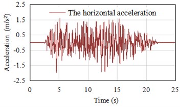
a) Horizontal acceleration time history PGA = 1.973 m/s2
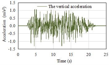
b) Vertical acceleration time history PGA = 1.315 m/s2
Fig. 9The retrieved acceleration time history (Horizontal direction PGA = 1.756 m/s2)
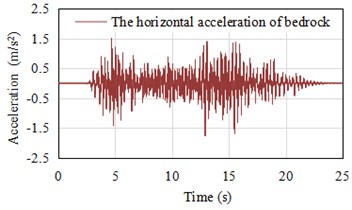
Three direction accelerations are directly put on massless foundation model 1 and 2 during a seismic time-history response; the model 3 to 5 used the viscoelastic boundary, the acceleration time history of the bedrock was inversion from the ground. After the acceleration adjusted and filtered, the displacement and velocity are obtained by integration, and the equivalent load on each node is obtained by using the program based on wave theory.
4. Seismic dynamic response analysis
4.1. The displacement of intake tower
Deformation of the intake tower is an important refer in seismic response. Three directions’ displacement of the five intake tower models listed in Table 4.
As can be clearly seen from Table 4, except the displacement along river flow direction of model 1, the maximum displacement values of the viscoelastic artificial boundary model (Model 3 to 5) are generally lower than the massless foundation models (Model 1 and 2), especially in the cross-flow direction the maximum reduced up to 80 %. The maximum displacement value of each direction occurrences slightly delayed than the input acceleration peak time of models without contact, and the peak value appearance time of contact models is not necessarily near the time of the input acceleration, the contact models’ displacement generally greater than the models without contact. This is because of the intake tower and the surrounding rock and foundation are a whole, the deformation of the intake tower restricted by surround rock, but the models with contact intake tower and surrounding rock may disengage during an earthquake, the deformation range of the tower body becomes larger which is closer to the fact that the intake tower and the backfill are not fully consolidated.
Model 5 set the viscoelastic boundary, but the free surface before the tower as the reflective face for wave propagation. It can be seen that the displacement value is greater than the model 3 or 4 that also using viscoelastic boundary, but it is little less than the model of massless foundation. The results show that the model 5 can be a certain extent embodies of the effects of radiation damping of infinite foundation, and the result is better than massless foundation method.
Table 4The absolute maximum displacement and occurred moment of each direction of the intake tower
Model name | Along river flow direction | Cross river flow direction | Vertical | |||
Displacement (cm) | Occurrence time (s) | Displacement (cm) | Occurrence time (s) | Displacement (cm) | Occurrence time (s) | |
Model 1 | –2.55 | 5.28 | –3.82 | 6.76 | –1.06 | 5.27 |
Model 2 | 4.49 | 14.02 | –4.93 | 9.47 | 1.48 | 14.03 |
Model 3 | –3.27 | 13.71 | 0.78 | 11.01 | –1.11 | 13.69 |
Model 4 | –3.85 | 14.29 | 1.51 | 7.27 | –0.92 | 13.81 |
Model 5 | 4.03 | 15.13 | –2.98 | 13.73 | –1.48 | 13.69 |
4.2. The stress of intake tower
Maximum principal stress and occurred moment of the intake tower of five models are listed in Table 5.
Seen from the Table 5 and Fig. 10, the maximum value of the stress located in the connection parts of the tower and the surrounding rock, the material is not considered nonlinear so that the value of the resulting stress is larger. The results of the five models are compared: The absolute maximum value of the model of the massless foundation is larger than that of the model 3 and model 4. The stress value of the contact model is obviously smaller than that of the model without contact. Model 4’s maximum value of the first principal stress decreased by nearly 57 % than model 1’s, it proves that the model used viscoelastic boundary with contact can effectively weaken the reflection of energy in the foundation, and the stress can release at the tower and the surrounding rock connect part. The maximum stress occurred at the same time for model 5 and model 3, but stress value of model 5 is greater than other models, so this set of viscoelastic boundaries cannot dissipate energy even increased the structure response. It proves that reasonable selection of viscoelastic boundary reflection faces has significant influence to result.
Table 5Maximum principal stress and occurred moment of the intake tower
Model name | Maximum value of first principal stress | Minimum value of Third principal stress | ||
Stress (MPa) | Occurrence time (s) | Stress (MPa) | Occurrence time (s) | |
Model 1 | 13.02 | 5.26 | –12.53 | 5.06 |
Model 2 | 11.03 | 14.02 | –11.82 | 14.01 |
Model 3 | 8.88 | 5.35 | –11.9 | 5.17 |
Model 4 | 5.66 | 14.31 | –7.93 | 14.31 |
Model 5 | 16.13 | 5.35 | –18.23 | 5.17 |
4.3. The acceleration changes along the height of intake tower
In order to compare the acceleration changes along the height of intake tower under different boundary conditions, model 3 to 5 were selected as the study object. ABCD four measuring points were set to observe the change of acceleration distribution along the height of intake tower, these points’ position was shown in Fig. 11(a). Point A at the top of intake tower, point B is located between point A and point C, point C at the demarcation line between tower and backfill and point D at the bottom of intake tower. Make the coordinate zero point at point D, when the maximum acceleration value of point A was appearing, then get the acceleration results from point B, C and D for model 3 to model 5, the acceleration distribution along the tower was obtained. Fig. 11(b).
Seen from the Fig. 11(b): point D to C, the acceleration value between models have litter alter from point D to C, this is due to the CD segment of the tower close to the back mountain, the acceleration along the height is difficult to amplify. From point C to A, the acceleration of three models are increased in a line tread, and the maximum of acceleration from model 3 to 5 is 7.51 m/s2, 5.11 m/s2, 11.63 m/s2. The viscoelastic boundary is adopted in this paper with contact the smallest increase along the height of the acceleration, and the largest increase in model 5. For three models, the acceleration ratio of point A to C is 15.9, 7.4 and 28.5. The above comparison also shows that the load input method and the contact boundary conditions have significant influence on the results of dynamic analysis of intake tower.
Fig. 10Maximum principal stress of the intake tower
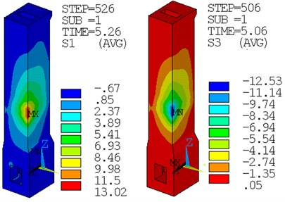
a) The first and third principal stress of model 1, Unit: MPa
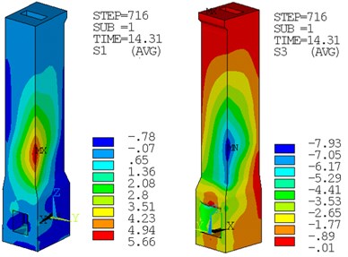
b) The first and third principal stress of model 4, Unit: MPa
Fig. 11Acceleration along the intake tower height distribution
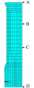
a) Schematic diagram of analysis point
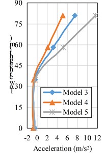
b) Distribution of acceleration along height
4.4. The contact state of intake tower
For model 4, the contact state for the contact area is observed. In the whole process of the earthquake, the bottom of the tower and the foundation has been in a closed state of adhesion.
Some parts of two sides of the intake tower cracked but in contact state during earthquake, crack position changes with time, the initial cracking part is mainly at the two sides of the bottom of the base plate, the cracking range extends from the back of the base plate to the middle-front region; but other parts recovery to adhesion state when cracking Fig. 12(a).
At the time of 14.07 s, the part that two flanks of the intake tower at the body shape contraction rear back is cracked, but the crack does not extend to the lower part or the upper part, these instructions that they still have good consolidation between the tower and the surrounding rock except small parts are cracking and contacting.
The front face has good adhesion between the intake tower and the rock during the earthquake. The behind sides of tower ship or cracking at six moments. Cracking at the highest boundary line of the surrounding rock behind the tower and cracks expand to the lower part over time, the deepest location of the cracking was achieved in 14.31 s Fig. 12(b), the upper contact adhesion state recovery.
Fig. 12Contact status of both sides and rear side of the intake tower
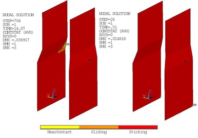
a) The contact states of both sides of the intake tower at 14.07 s and 0.51 s
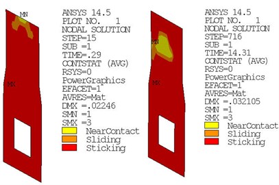
b) The contact states of back of intake tower at 0.29 s and 14.31 s
From the analysis above, in the design earthquake, although around the intake tower have some crack, no penetrative disengage in the model, even after cracked it still in the contact state, and only small range in the cracking position and other cracked locations restores adhesion state at every time, it can be concluded that intake tower without sliding or overturning, its stability meets the request.
5. Conclusions
Based on the previous viscoelastic boundary research, proposed the method of viscoelastic boundary applies for abrupt step topography, through a small example to verify the correctness of the program and using the method to dynamic analysis for an intake tower in hydropower station. The displacement and stress of the tower under the condition of massless foundation and contact condition are compared. The given method may be applied to the dynamic analysis of bank-tower intake with homogeneous foundation. Some conclusions are given as follows:
1) When the ground surface has obvious hypermutation, viscoelastic artificial boundary should be applied to the calculation of sub-regional node load, this displacement is to be enlarged at the volley surface of highly abrupt, its value greater than the incident and reflected superposition value.
2) The contact relationship between the intake tower and the surrounding rock and the foundation should be considered. The state that closed, separation or sliding between the tower and the surrounding rock can represent during an earthquake. And also, set contact elements can release the tensile stress and reduce the acceleration value along the tower height, this is much closer to reality.
3) In practical engineering, bank-tower intake as a common form of water inlet, it back to the mountain so has good stability, but the slope of mountain will be cut when construction, thus forming a steep terrain. The results of this study show that the influence of step topography must be taken into account, and the reasonable viscoelastic boundary setting and load input are made.
References
-
China Renewable Energy Engineering Institute. Code for Seismic Design of Hydraulic Structures of Hydropower Project (NB 35047-2015). China Electric Power Press, Beijing, China, 2015.
-
Yin G. H., Chen Q. J. Inversion of ground motion and analysis of soil-structure dynamic interaction. Chinese Quarterly of Mechanics, Vol. 31, Issue 2, 2010, p. 256-264.
-
Pak R. Y. S., Ji F. Mathematical boundary integral equation analysis of an embedded shell under dynamic excitations. International Journal for Numerical Methods in Engineering, Vol. 37, Issue 14, 1994, p. 2501-2520.
-
Eskandari M., Ahmadi S. F., Khazaeli S. Dynamic analysis of a rigid circular foundation on a transversely isotropic half-space under a buried inclined time-harmonic load. Soil Dynamics and Earthquake Engineering, Vol. 63, Issue 1, 2014, p. 184-192.
-
Ahmadi S. F., Eskandari M. Vibration analysis of a rigid circular disk embedded in a transversely isotropic solid. Journal of Engineering Mechanics, Vol. 140, Issue 7, 2013.
-
Pak R. Y. S., Guzina B. B. Seismic soil-structure interaction analysis by direct boundary element methods. International Journal of Solids and Structures, Vol. 36, Issue 31, 1999, p. 4743-4766.
-
Pak R. Y. S., Guzina B. B. Three-dimensional Green’s functions for a multilayered half-space in displacement potentials. Journal of Engineering Mechanics, Vol. 128, Issue 4, 2002, p. 449-461.
-
He X. L., Li T. C. Dynamic artificial boundaries condition for infinite domain. Advances in Science and Technology of Water Resources, Vol. 25, Issue 3, 2005, p. 64-67.
-
Liu J. B., Lu Y. D. A direct method for analysis of dynamic soil-structure interaction based on interface idea. Developments in Geotechnical Engineering, Vol. 83, Issue 3, 1998, p. 261-276.
-
Gao W. T. Nonlinear Seismic Analysis of Intake Tower of Hydropower Station. Master’s Thesis, Xi’an University of Technology, Xi’an, China, 2011.
-
Chen Z., Xu Y. J. Nonlinear finite element analysis of high intake tower based on wave motion theories. China Civil Engineering Journal, Vol. S1, Issue 43, 2010, p. 560-566.
-
Liu J. B., Wang Z. Y., Du X. L. Three-dimensional visco-elastic artificial boundaries in time domain for wave motion problems. Engineering Mechanics, Vol. 22, Issue 6, 2005, p. 46-51.
-
Zhao R. B., Zhang J. J., Liu Z. X., et al. Analysis of seismic wave problem based on visco-elastic artificial boundary under the ladder terrain. World Earthquake Engineering, Vol. 3, 2015, p. 220-227.
-
Jiang X. X., Li J. B., Lin G. Study on the seismic input mode of viscoelastic artificial boundary under the condition of slope site. World Information on Earthquake Engineering, Vol. 29, Issue 4, 2013, p. 126-132.
-
Chen Z., He S. H. Wave-motion theory based simulation analysis on height of backfill for rear of intake tower. Water Resources and Hydropower Engineering, Vol. 43, Issue 3, 2012, p. 35-37.
-
Kong K., Feng G., Fan C. Z. Effects of backfill height of intake tower back on its static and dynamic performances. Engineering Journal of Wuhan University, Vol. 44, Issue 2, 2011, p. 192-196.
-
Li N., Li Q., Ren T. Dynamic response analysis of zipingpu intake tower under wenchuan earthquake action. Chinese Journal of Underground Space and Engineering, Vol. 10, Issue 5, 2014, p. 1127-1134.
-
Shi G. B. Influence of mechanics model of intake tower foundation contact surface on tower structural stress. Northwest Hydropower, Vol. 6, 2010, p. 63-66.
-
Liu J. B., GU Y., Du Y. X. Consistent viscous-spring artificial boundaries and viscous-spring boundary elements. Chinese Journal of Geotechnical Engineering, Vol. 28, Issue 9, 2006, p. 1070-1075.
-
Zhang P. Z., Xu X. W., Wen X. Z., et al. Slip rates and recurrence intervals of the Longmen Shan active fault zone, and tectonic implications for the mechanism of the May 12 Wenchuan earthquake, 2008, Sichuan, China. Chinese Journal of Geophysics, Vol. 51, Issue 4, 2008, p. 1066-1073.
-
Xie Z. T., Zhang J. F., Tian Y., et al. Research on inversion of earthquake acceleration time-period from ground to interior stratum. Journal of Xian University of Technology, Vol. 23, Issue 4, 2007, p. 418-421.
-
Liang J. W., Ba Z. N. Surface motion of a hill in layered half-space subjected to incident plane SH waves. Journal of Earthquake Engineering and Engineering Vibration, Vol. 28, Issue 1, 2008, p. 1-10.
-
Hao M. H., Zhang Y. S. Analysis of the adjacent terrain effect on the properties of ground motion. Earthquake Research in China, Vol. 36, Issue 5, 2014, p. 883-894.
-
Ding Z. H., Zhou H., Jiang H. Effect of 3-D step topography on ground motion. Acta Seismologica Sinica, Vol. 36, Issue 2, 2014, p. 184-199.
-
Liu Y. H., Zhang B. Y., Chen H. Q. Comparison of spring-viscous boundary with viscous boundary for arch dam seismic input model. Journal of Hydraulic Engineering, Vol. 37, Issue 6, 2006, p. 758-763.
About this article

This work was supported by National Natural Science Foundation of China (No. 51179154).
