Abstract
In modal testing, the force transducer and accelerometer mounted on the test structure will introduce extra mass effects to the system and then affect the measured Frequency Response Functions (FRFs). This paper proposed a method for assessing sensor mass effects on the measured FRFs in shaker modal testing. The assessment method offers some distinct advantages where very few FRFs measurements are required, and more importantly it does not require calculations involving several measured FRFs, hence avoiding further contaminations of the measured data. In view of two different ways of response measurements, two cases have been discussed: (1) shaker + laser Doppler vibrometer and (2) shaker + accelerometer. In case (1), only force transducer mass need be assessed. In case 2, however, both force transducer and accelerometer masses should be considered. Especially in Case 2, the overall as well as the individual mass effects of the two transducers were assessed. It is found that the assessment method is quite effective in the experimental validation for Case 1. A simple numerical example for Case 2 presented also illustrates the good theoretical performance of the method. The same example is extended to incorporate simulated noise, simulating an experimental situation, and it is shown that the accuracy of assessment results will be affected to some extent by the noise. It is suggested that the measured FRFs be preprocessed using the curve-fitting procedure before applying the proposed method.
1. Introduction
In modal testing, the measured Frequency Response Functions (FRFs) are often inaccurate due to the transducers mass effects [1-6]. Clearly, lighter transducers are preferable, however, they have a high cost and are not always available. Furthermore, even small (or lightweight) transducers may also introduce great mass effects when the test structures are small and flexible. Some correction methods of removing transducer mass effects from the measured FRFs have been investigated in [7-13]. Generally, these correction methods have some points in common in that several FRFs have to be measured and be involved in the calculations. Moreover, a significant point is that the correction accuracies of these methods are to a different extent sensitive to the noise, thus weakening their performance in the practical application. Inevitably, any transducers mounted on the structures will more or less introduce extra masses to the system and then change their dynamic characteristics. However, the mass effects are not significant in all the tests. Especially in the test in which the mass ratio of transducer and test structure is very small, the transducer mass effects are negligible. These insignificant mass effects are generally ignored intentionally rather than being corrected so as to improve the efficiency of the modal test. Thus, it is suggested that “obvious” mass effects be corrected and the “negligible” be ignored in the engineering practice. But how to judge the mass effects “obvious” or “negligible”? So far, it generally relies on the empirical judgment of engineers, or according to the mass ratio of the transducer and test structure. However, even in the case of the same mass ratio, transducer mass effects vary with different sensor mounting positions [14]. Moreover, even with the same sensor installation location and same mass ratio, the mass effects on different orders of modal are not the same. Therefore, the quality of transducer mass effects cannot be judged empirically. It depends on the magnitude of transducer mass, mass ratio of the transducer and test structure, installation position of the transducer and modal order. In order to properly process the transducer mass effects in engineering (“correct” or “neglect”), a quick method for assessing transducer mass effects on the measured FRFs is essential.
From a practical point of view, a comparison between the natural frequencies of the measured FRF and those of the exact FRF is a suitable criterion for assessing the quality of the transducer mass effects [15]. When there is no discernible change in the natural frequency of the structure due to the attachment of the transducer, the measured FRFs can be judged to have a good quality. Otherwise, the results are not reliable, and there is a necessity to remove the transducers mass effects from the measured FRFs. Therefore, to assess the transducer mass loading effect, the main task is to obtain the natural frequencies of the measured FRFs and exact FRFs, respectively. The first ones can usually be easily acquired from conventional measurements of FRFs; however, the later ones are often difficult if it is not impossible to access them from an experimental test. Ashory [15] investigated a method of assessing the mass-loading effects of accelerometers by using an extra mass with the same mass as that of the accelerometer. The current authors presented a quick method for assessing transducer mass effects on the measured FRFs in an earlier work [16], and this article expands on that work with additional theoretical results and illustrates the theory with modeling as well as experiments.
This method firstly predicts the natural frequencies of the exact FRFs (corresponding to original structure) based on the measured FRFs, and then assessing the quality of the transducer mass effects by comparing the natural frequencies of the exact and measured FRFs. Some advantages of the proposed method are: (1) very few FRFs measurements are required, and more importantly (2) it does not require calculations involving several measured FRFs, hence avoiding further contaminations of the measured data. In what follows, the overall as well as the individual mass effects of two transducers (force transducer and accelerometer) were assessed. In literature [7], correction of transducer mass effects from the measured FRFs in the two cases has been discussed. The assessment methods in this paper are based on some theory conclusions of the correction methods given in [7].
2. Assessment of transducer mass effects on measured FRFs
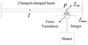
Fig. 1 shows the force transducer mass effects on a clamped-clamped beam. According to [1], the point FRF and transfer FRF can be corrected by employing Eq. (1) and (2), respectively:
where and App are measured and exact point FRFs, respectively. and are measured transfer and exact FRFs.
Fig. 1Force transducer mass effects on clamped-clamped beam
Eq. (1) and (2) perform perfectly in theoretical conditions, however, their practical applications are usually not satisfactory due to the noise pollution in FRFs measurements. When the measured FRFs and are contaminated with noise, the multiplication and division operations in Eqs. (1) and (2) will further amplify the noise effects on the results of and . Thus, the corrected results and will be affected and the natural frequencies extracted from (or ) may be inaccurate.
A new approach of predicting the exact natural frequencies is presented here in some other way. It is obvious that both and have natural frequencies at where and have their local maximum amplitudes. Note that here refers to a set of natural frequencies (corresponding with different orders) of the original structure. Making a further investigation of Eq. (1) and (2), we will find that will make the denominator of Eqs. (1) and (2) approximate to zero. Especially when the system under consideration is undamped, will make the denominator of Eqs. (1) and (2) equal to zero. By equating the denominator of Eqs. (1) and (2) to zero and then solving the resulting equation, one yields:
With respect to Eq. (3), the graphical method is utilized here for the convenience in practical application. It means that if is drawn on a graph together with , the frequencies at their intersection points can be considered as the natural frequencies (denoted as ) of the original structure. It should be mentioned that is complex and its module is used as the plot data. If the natural frequencies of and are denoted as , the mass effect of force transducer can then be assessed by the comparison of and . For example, if the first mode is our concern, the mass effects can be quantified by:
If the value of is less than the allowed error, it can be considered that the transducer mass effects are not apparent and can be ignored. Otherwise, the original measured FRFs are not acceptable and should be corrected by employing Eqs. (1) and (2).
Note that the assessment method is just right applicable for case 1: shaker + laser Doppler vibrometer modal testing in which only force transducer mass effects are involved. Details for this case are discussed in section 2.1.
2.1. Case 1: shaker + laser doppler vibrometer
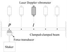
Laser Doppler vibrometer is welcome in shaker modal testing for the very advantage of non-contact measurement that will not introduce extra mass effects to the test. It is scanned sequentially from one point to another one to measure the response of the different points. The implementation regarding to the case 1 can be seen in Fig. 2.
Fig. 2Shaker + laser doppler vibrometer measurement
In view that Doppler vibrometer is commonly used to measure a velocity signal. However, the FRF in Eq. (3) refers to accelerance. This presents no complication since accelerance and velocity FRF can be transformed into each other. By dividing both sides of Eq. (3) by , we can easily get:
where is the measured velocity point FRF. As only one point FRF measurement is required, Eq. (5) is very practical for the assessments of the transducer mass effects on the measured FRF in shaker + Laser Doppler vibrometer modal testing. Note that the transducer mass effects on the point FRF are identical to that on the transfer FRFs. This is because the force transducer is installed at the same point throughout the point FRF and transfer FRFs measurements. It means that the structure has not been changed during the point FRF and transfer FRFs measurements. Therefore, the measured point FRF and transfer FRFs (corresponding to modified structure) have the same natural frequencies . And the exact point FRF and transfer FRF (corresponding to original structure) also have the same natural frequencies . Both the mass effect on point FRF and transfer FRFs can then be assessed by the comparison of and .
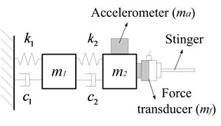
2.2. Case 2: shaker + accelerometer
In case 2, both the force transducer and accelerometer will affect the measured FRFs. The overall mass effects of the two transducers can then be assessed by a comparison of the natural frequencies of the exact FRF and those of the measured FRF. Note that the transducers mass effects on the point FRF are different from that on the transfer FRFs due to the varying location of the accelerometer. Thus, the assessments of transducers mass effects on point FRFs and transfer FRFs are respectively discussed in the following two Sections (2.2.1 and 2.2.2). Besides, sometimes it may also be required to assess the individual mass effects of the two transducers. For example, to assess the force transducer mass effects, it requires a comparison of the natural frequencies of the exact FRF and those of a “special FRF” in which only force transducer mass is involved. Therefore, in each Section (2.2.1 and 2.2.2), the overall as well as the individual mass effects of the two transducers are assessed.
2.2.1. Assessment of mass effects on point FRF
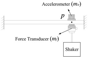
This situation presents no complication when the point FRF is assessed because the response co-ordinate coincides with the shaking point, as shown in Fig. 3. The two-transducers masses can be considered as an integrated mass. By replacing with () in Eq. (3), we can easily obtain Eq. (6) from which the natural frequencies of the exact FRF can be predicted. If natural frequencies of the measured FRFs are denoted as , the overall masses effects of the two transducers can be assessed by the comparison of and . Note that and denotes force transducer and accelerometer mass effects, respectively:
To assess the force transducer mass effects separately, we should obtain the natural frequencies (denoted as ) of point FRF which is the “special FRF” mentioned above. This situation becomes complicated since is not available from a straightforward measurement. To obtain , a similar method as that of predicting the exact natural frequency (see Eq. (3)) is utilized again. First, is derived by employing the mass correction method [7, 8] (removing the accelerometer mass effects from ), as shown in Eq. (7):
It can be found that has natural frequencies at that make the denominator of Eq. (7) approach zero. By equating the denominator of Eq. (7) to zero and then solving the resulting equation, one yields:
Then, can be easily obtained according to Eq. (8) by the graphical method. Thus, the mass effects of force transducer can be assessed by the comparison of and .
Similarly, to assess the accelerometer mass effects individually, can be obtained by removing the force transducer mass from :
where is point FRF in which only accelerometer mass is involved. Likewise, has natural frequencies at that make the denominator of Eq. (9) equal to zero and then solving the resulting equation, one yields:
Then, accelerometer mass effects can be assessed by the comparison of and .
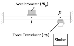
Fig. 3Measuring point FRF App(p1,p2)
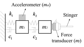
2.2.2. Assessment of mass effects on transfer FRFs
The discussion in the previous section indicates that the mass effect on point FRFs is the same as that on transfer FRFs in case 1. In case 2, however, the mass effects are changing due to the movement of the accelerometer for different transfer FRFs measurement. Assuming the natural frequencies of to be , the total mass effects of the two transducers on the measured transfer FRF can be assessed by the comparison of and which can be readily obtained from Eq. (6).
The situation becomes more complicated when the two-transducers mass effects on the measured transfer FRFs are separately assessed. To assess accelerometer mass effects, we should first get the natural frequencies of transfer FRF in which only accelerometer mass is involved. Since is also not available from the straightforward measurement, the mass correction method is utilized again. can be obtained by removing the force transducer mass effects from , as shown in Eq. (11):
Unfortunately, is still unachievable as in Eq. (11) cannot be measured directly. Correction method is utilized again, and can be obtained by removing the accelerometer mass effects from , as it can be seen in Eq. (12):
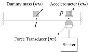
It should be noted that is measured with a dummy mass (equals the mass of the accelerometer ) attached to point , as shown in Fig. 5.
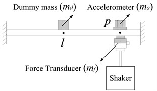
Fig. 4Measurement of transfer FRF Alp(p1,l)
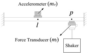
Fig. 5Measurement of point FRF App(p1,p2,l)
Substituting Eq. (12) into Eq. (11), one yields:
Thus, has natural frequencies at that make the denominator of Eq. (13) approach zero and then solving the resulting equation, one yields:
Thus, can be obtained from Eq. (14). Then, the accelerometer mass effects on the measured transfer FRF can be assessed by the comparison of and which can be readily obtained from Eq. (6). So far, the quality of accelerometer mass effects on the measured transfer FRF has been assessed.
To assess force transducer mass effects separately, we should first get the natural frequencies of transfer FRF in which only force transducer mass gets involved. The situation of measuring is contradictory since the accelerometer mass should not be attached (at point l), while, the measurement cannot be performed without the accelerometer. Fortunately, the transfer FRF have the same natural frequencies as those of the point FRF which are already available from Eq. (8). Thus, the natural frequencies of can also be predicted using Eq. (8).
Besides, some researchers have investigated the mass correction methods which can also be employed here to obtain by removing the accelerometer mass from the measured transfer FRF . Two different methods have been discussed by Carkar [8] and Ashory [11], respectively. According to the measurement scheme in Fig. 6 given in [8], can be acquired by removing the accelerometer mass effects from using Eq. (15):
The detailed measurement process is as follows:
• Measuring point FRF according to Fig. 3,
• Measuring transfer FRF according to Fig. 6(a),
• Measuring point FRF according to Fig. 6(b).
It should be noted that the chosen dummy mass equals the accelerometer mass in Fig. 6.
The accelerometer mass can then be removed from the measured transfer FRF according to Eq. (15).
Fig. 6Measurements using accelerometers and dummy mass
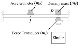
a) Measurement of
b) Measurement of
In Eq. (15), has natural frequencies at that make the denominator of Eq. (15) approach zero and then solving the resulting equation, one yields:
Thus, the natural frequencies of can be predicted from Eq. (16). It is not surprising that the Eq. (16) coincides with Eq. (8) which is previously mentioned for predicting the natural frequencies of .
According to literature [11], the mass effects of accelerometer can be eliminated from the using Eq. (17), see Fig. 7:
where and are measured according to Fig. 7(a) and (b), respectively. is corrected transfer FRF after removing the mass effects of accelerometer.
Fig. 7Repeated measurement of transfer FRF using two accelerometers with different masses

a)
b)
Thus, has natural frequencies at that make the denominator of Eq. (17) approach zero and then solving the resulting equation, one yields:
Thus, can also be obtained from Eq. (18). And it can be seen that both Eq. (16) (or Eq. (8)) and (18) can be employed to obtain the natural frequencies of .
Table 1Conclusion of assessment method
FRFs to be assessed | Transducers involved | Natural Frequencies to be compared | FRFs required to be measured | |
Case 1: Shaker + laser Doppler vibrometer | Point FRF | Force transducer | , | |
Transfer FRF | Force transducer | , | ||
Case 2: Shaker + accelerometer | Point FRF | Force transducer | , | |
Accelerometer | , | |||
Two transducers | , | |||
Transfer FRF | Torce transducer | , | or ( and ) | |
Accelerometer | , | , | ||
Two transducers | , | , |
So far, assessments of transducer mass effects on both point and transfer FRFs have been investigated. Besides, the overall as well as individual mass effects of two transducers have been assessed, respectively. The conclusions are given in Table 1.
3. Verification of assessment method
3.1. Experimental validation for case 1: shaker + laser doppler vibrometer
A clamped-clamped beam is chosen as the test object in this case, shown in Fig. 8. The density and dimensions of the beam are 7.8 g/cm3 and 400×50×5 mm3, respectively. The force transducer mass is 0.025 kg and there is no acceleration sensor involved in this test. Nine measurement points are evenly arranged along the longitudinal direction of the beam. And the exciting is fixed at point 5 while the response measurement is varied sequentially from point 1 to point 9. To assess the mass effects, we should first predict the natural frequencies of the exact point FRF according to Eq. (5) and then compare the predicted natural frequencies with those of the measured FRF . However, the correctness of the predicted natural frequencies cannot be judged since the exact dynamics of the supported beam are not known to us in advance. Therefore, the effectiveness of the assessing method cannot be evaluated. To solve this problem, two sets of experiments are conducted in this study. Detail of the experiments design can be found in [7].
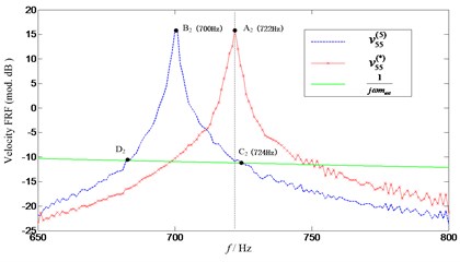
Firstly, FRF (without extra mass ) and (with extra mass 0.025 kg) are measured, respectively. Then the natural frequencies of target FRF can be obtained using Eq. (5). Since the exciting point 5 is located at the middle of beam, the second resonance is not excited and only the first and third resonance frequencies are exhibited, as it can be seen from Fig. 9. What’s more, the curves of and 1 intersected at some points, as expected. As clearly shown in Fig. 10, the curves with respect to and 1 intersect at two points ( and ). However, point is the only solution we are expecting. This is due to the fact that the curve of (which is complex) is figured using its absolute value, which makes one more intersection appear. As known to all of us, the natural frequencies of the affected structure (with the extra mass attached) should be lower than those of the unaffected original structure (without the extra mass attached). Therefore, the frequency of point which is lower than that of point (corresponding with the natural frequency of ) should be excluded from the solutions. Furthermore, the predicted natural frequency (see point at 96 Hz) is consistent with that of the target FRF (see point at 96 Hz), which demonstrated the effectiveness of the proposed method. Similar observations can also be made for the third natural frequency illustrated in Fig. 11. Somewhat deficient is that the predicted third frequency (724 Hz) deviates slightly from that of the target one (722 Hz). This is due to the noise contamination in the measurement and the curve of the measured FRF in frequency bands 650-800 Hz is not as smooth as that in 50-150 Hz. However, this small deviation (between and ) is acceptable compared with that between and . From the mass effects assessment, it can be found that a 4 Hz change in the first natural frequencies of the beam is little and can be ignored. However, for the third natural frequency, an error of 24 Hz is too large to be negligible.
Fig. 8Shaker modal testing of clamped-clamped beam using Laser doppler vibrometer
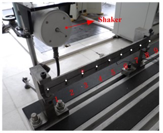
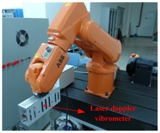
Fig. 9Comparison of curves of v55(5), 1/jωmext and v55(*)

Fig. 10Comparison of predicted and target first natural frequency
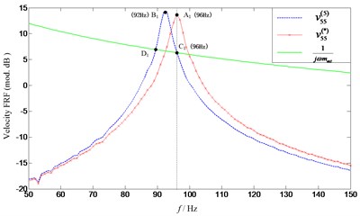
Fig. 11Comparison of predicted and target third natural frequency
3.2. Numerical simulation study for case 2: shaker + accelerometer
A two-degrees-of-freedom simulated modal testing system shown in Fig. 12 was presented for the verification of the proposed method. The system parameters are given in Table 2. The “measured” accelerances matrix is numerically generated according to Eq. (19):
where is accelerances matrix. And , and are mass, stiffness and damping matrixes which are assembled by employing the system parameters given in Table 2.
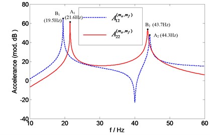
Then accelerances and can be extracted from the matrix, and their curves are shown in Fig. 13.
Fig. 12Simulated modal testing
a) Measuring
b) Measuring
Generally, the driving point FRF and transfer FRFs of the same system should have the same resonance frequencies. In Fig. 13, however, the resonance frequencies of the point accelerance are inconsistent with those of the transfer accelerance . This is due to the fact that the accelerometer is attached at different points when the point FRF and transfer FRF are measured. Thus, the accelerometer mass effects on point accelerance are different from that on transfer accelerance .
Table 2System parameters
0.3 Kg | 0.1 Ns/m | 12000 N/m | 0.06 Kg | 0.05 kg |
0.1 Kg | 0.12 Ns/m | 7000 N/m | 0.08 Kg |
Fig. 13The “measured” point accelerance A22(ma, mf) and transfer accelerance A12(ma, mf)
3.2.1. Assessing the transducer mass effects on point accelerance
According to the proposed method, only the measurement of point accelerance is required to predict the natural frequencies of , , and , hence assessing the force accelerometer, transducer and their overall mass effects on the measured point accelerance , respectively. The overall mass effects of the two transducers can be assessed by comparison of the natural frequencies of the “measured” accelerance and those of the exact accelerance . According to Eq. (6), the natural frequencies of can be acquired by searching the intersection points of and 1. As is shown in Fig. 14, the curves of and 1 intersect at points , and , . However, and are excluded from the solutions by the common sense that the natural frequencies of (without transducers attached) should be higher than those of (with transducers attached). Thus, the remaining points (25.7 Hz) and C2 (52.1 Hz) correspond with the first and second natural frequency of , respectively. For comparison purpose, the exact accelerance is also numerically generated in Fig. 14. And it can be found that the resonances frequencies (25.7 Hz) and (52.1 Hz) of are in a quite good agreement with the predicted ones (25.7 Hz) and (52.1 Hz), which demonstrate the effectiveness of the proposed method.
Similar observations can also be made for the assessment of the individual mass effects of accelerometer and force transducer illustrated in Fig. 15 and Fig. 16. In Fig. 15, the natural frequencies of can be found at the intersection points ( (21.7 Hz) and (46 Hz)) of and 1. And the natural frequencies of can be found at the intersection points ( (22.6 Hz) and (46.9 Hz)) of and 1, as it can be seen in Fig. 16.
Table 3 shows the shifts of natural frequencies of point accelerance due to the transducer mass effects. In this table, the second, third and forth columns correspond with natural frequencies shifts caused by the accelerometer, force transducer and their overall mass loading effects, respectively. The natural frequencies shift in the fourth column indicate the quantity of the transducers masses effects in shaker accelerometer modal testing (the mass of both two transducers is involved). And the second column can be considered as the accelerometer mass effects in hammer + accelerometer testing (only accelerometer mass is involved). The third column can be considered as force transducer mass effects in shaker + Laser Doppler vibrometer modal testing (only force transducer mass is involved). It can be predicted from the second and third column that if this system is respectively tested in hammer + accelerometer and shaker + Laser Doppler vibrometer cases, the mass effects of accelerometer in the former are larger than that of force transducer in the later. This is due to that the mass of the acceleration sensor is larger than that of the force sensor, and two sensors are installed in the same location.
Fig. 14Prediction of natural frequencies of A22 for assessing overall mass effects of two transducers
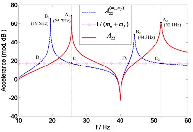
Fig. 15Prediction of natural frequencies of A22(ma) for assessing accelerometer mass effects
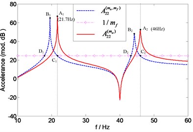
Fig. 16Prediction of natural frequencies of A22(mf) for assessing force transducer mass effects
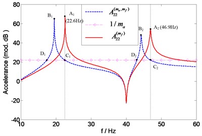
Table 3Shift of natural frequencies (Hz) of point accelerance A22 due to accelerometer, force transducer, and their overall mass effects
Accelerometer | Force transducer | Overall | |
First order | 4.0 | 3.1 | 4.1 |
Second order | 6.1 | 5.2 | 8.4 |
3.2.2. Assessment of transducer mass effects on transfer accelerance
The overall mass effects of the two transducers on the transfer accelerance can be assessed by a comparison of the natural frequencies of the “measured” accelerance and exact accelerance . This presents no complication since the natural frequencies of are the same as those of which are readily acquired in the previous discussion. Thus, the natural frequencies of can also be found at the intersection points ( (25.7 Hz) and (52.1 Hz)) of and 1, as shown in Fig. 17.
To assess the individual mass effects of accelerometer, an extra measurement of point FRF is required to predict the natural frequencies of according to Eq. (14). As shown in Fig. 18, and 1 intersect at points (24 Hz) and (49.7 Hz) which correspond with the first and second natural frequency of , respectively. The force transducer mass effect on the transfer accelerance can be assessed by a comparison of the natural frequencies of the “measured” accelerance and those of the exact accelerance . The natural frequencies of A12 are identical with those of A11 which are readily obtained before. Since has the same natural frequencies as , the natural frequencies of can also be found at the intersection points ( (22.6 Hz) and (46.9 Hz)) of and 1, as it can be seen from Fig. 19. It is not surprising that the same results (intersection points (22.6 Hz) and (46.9 Hz) in Fig. 20) can also be obtained by employing another method (using two accelerometers with different masses, see Eq. (18)). For the comparison purpose, , and are numerically calculated and also shown in Figs. 17-20, respectively. It can be seen that the predicted natural frequencies are in a quite good agreement with the calculated ones.
Fig. 17Prediction of natural frequencies of A12 for assessing overall mass effects of two transducers
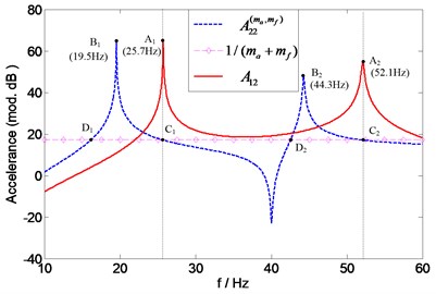
Fig. 18Prediction of natural frequencies of A12(ma) for assessing accelerometer mass effects
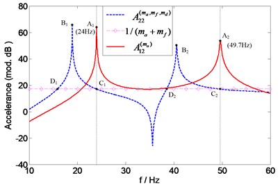
Fig. 19Prediction of natural frequencies of A12(mf) for assessing force transducer mass effects
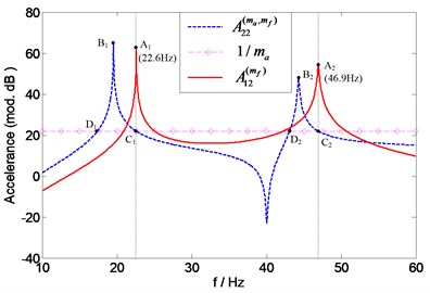
Fig. 20Prediction of natural frequencies of A12(mf) (using two accelerometers with different masses) for assessing force transducer mass effects
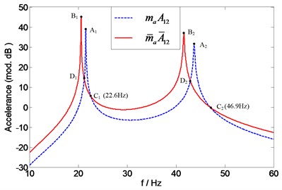
Table 4 shows the shifts of natural frequencies of transfer accelerance due to the transducer mass effects. It is not surprising to find that individual mass effects of force transducer on the transfer accelerance are identical to that on the point accelerance , as discussed before (see Table 1). However, compared with Table 3, a significant difference in Table 4 is that the individual mass effects of accelerometer are less than that of force transducer although the mass of accelerometer is larger than that of force transducer. This is primarily due to the fact that installation positions of the two sensors are different. It is further illustrated that the quality of transducer mass effects is not only related to magnitude of transducer mass, but also to installation location of transducer.
Table 4Shift of natural frequencies (Hz) of transfer accelerance A12 due to accelerometer, force transducer, and their overall mass effects
Accelerometer | Force transducer | Overall | |
First order | 1.7 | 3.1 | 6.2 |
Second order | 2.4 | 5.2 | 7.8 |
3.2.3. Discussion of methods with noisy data
It can be seen from the above discussion that the natural frequencies of , , and , , are needed for assessing the transducer mass effects on point and transfer accelerance, respectively. And a total of only two point FRFs and measurements are required to predict these natural frequencies. It means that the accuracy of the proposed assessment method depends largely on the measurement accuracy of and . The following simulations are presented to verify the effectiveness of the methods with noise-contaminated FRFs. The same system given in Fig. 12 is utilized here. The difference is that and are numerically incorporated with the white Gaussian noise (zero mean and variance ). The noise level is defined as:
where is the mean absolute value of in the frequency range of interest. The noise levels in this example are set to be 0.5 %, 1 %, respectively. Note that the FRF is a complex value; the random noise should be added to the real and imaginary parts of the FRF, respectively. The prediction results corresponding to 0.5 % noise are presented in Fig. 21.
Fig. 21Prediction of natural frequencies of A22 (0.5 % noise)
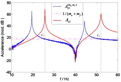
Fig. 22Prediction of natural frequencies of A22 (1 % noise)
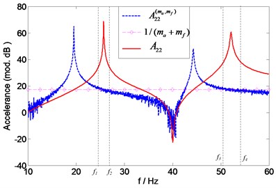
It is seen that the results ( and ) are less affected by the noise. This is because and 1 intersects at the points ( and ) corresponding to relatively large amplitudes which are contaminated less than the small amplitudes. With the noise level increasing to 1 %, the affected exhibits a lot of glitches. And several intersections points of and 1 being found in the frequency ranges and make it difficult to determine the accurate results (see Fig. 22). In this case, it is suggested that the measured FRFs be preprocessed using the curve-fitting procedure before the proposed assessment method is applied. The method may work well with the curve fitted data. Similar observations can also be made for predicting the natural frequencies of , and , . However, they are not presented here for sake of brevity.
4. Conclusions
The measured FRFs are often affected due to the mass of transducers mounted on the structure. This paper proposed a method for assessing transducer mass effects on the measured FRFs. The assessment is performed by comparing the natural frequencies of the measured FRF and those of the exact FRF. The conclusions are:
1) In Case 1: shaker + laser Doppler vibrometer, only one point FRF measurement is required for assessing the force transducer mass effects on point FRF and transfer FRF.
2) In Case 2: shaker + accelerometer, only one point FRF measurement is required to assess the transducer (whether force transducer or accelerometer or force transducer + accelerometer is used) mass effects on point FRF. And one point FRF measurement is needed to assess the force transducer mass effects on the transfer FRF; however, two point FRFs and should be measured when assessing the accelerometer mass effects on the transfer FRFs. Furthermore, one point FRF and one transfer FRF measurements are required for assessing the overall mass effects of the two transducers on transfer FRFs.
3) In both cases, the force transducer mass effect on point FRF is the same as that on transfer FRF. However, the accelerometer mass effect on point FRF is different from that on transfer FRF. This is because the force transducer is always fixed at a certain point in both cases, while, the accelerometer has to be moved to different locations for different transfer FRFs measurements in Case 2.
It is found that the assessment method is quite effective in the experimental validation for Case 1. A simple numerical example for Case 2 presented also illustrates the good theoretical performance of the method. The same example is extended to incorporate simulated noise, simulating an experimental situation, and it is shown that the accuracy of assessment results will be affected to some extent by the noise. It is suggested that the measured FRFs be preprocessed using the curve-fitting procedure before applying the proposed method.
References
-
Ewins D. J. Modal Testing: Theory, Practice and Applications. 2nd Edition, Research Studies Press, England, 2000.
-
Ewins D. J. Modal Testing: Theory and Practice. Research Studies Press, England, 1984.
-
Ole D. Prediction of transducer mass-loading effects and identification of dynamic mass. Proceedings of Ninth International Modal Analysis Conference, 1991, p. 306-312.
-
Mcconnell K. G. Vibration Testing: Theory and Practice. John Wiley and Sons Inc, New York, 1995.
-
Ren J., Wang J., Ting K., et al. Calibration of measured FRFs based on mass identification method. ASME 2015 International Design Engineering Technical Conferences and Computers and Information in Engineering Conference, 27th Conference on Mechanical Vibration and Noise, 2015, p. V8T-V13T.
-
Hossain N., Islam M. S., Ahshan K. N., et al. Effects on natural frequency of a plate due to distributed and positional concentrated mass. Journal of Vibroengineering, Vol. 17, Issue 7, 2015, p. 3751-3759.
-
Bi S., Ren J., Wang W., et al. Elimination of transducer mass loading effects in shaker modal testing. Mechanical Systems and Signal Processing, Vol. 38, Issue 2, 2013, p. 265-275.
-
Cakar O., Sanliturk K. Y. Elimination of transducer mass loading effects from frequency response functions. Mechanical Systems and Signal Processing, Vol. 19, Issue 1, 2005, p. 87-104.
-
Carkar O., Sanliturk K. Y. Elimination of noise and transducer effects from measured response data. Proceedings of ESDA 2002, 6th Biennial Conference on Engineering Systems Design and Analysis, 2002.
-
Silva J. M. M., Maia N. M. M., Ribeiro A. M. R. Cancellation of mass-loading effects of transducers and evaluation of unmeasured frequency response functions. Journal of Sound and Vibration, Vol. 236, Issue 5, 2000, p. 761-779.
-
Ashory M. R. Correction of mass-loading effects of transducers and suspension effects in modal testing. Proceedings of International Modal Analysis Conference, 1998, p. 815-828.
-
Silva J. M. M., Maia N. M. M., Ribeiro A. M. R. Some applications of coupling/uncoupling techniques in structural dynamics – part 1: solving the mass cancellation problem. Proceedings of 15th International Modal Analysis Conference, Vol. 2, 1997, p. 1431-1439.
-
Decker J., Witfeid H. Correction of transducer-loading effects in experimental modal analysis. Proceedings of 13th International Modal Analysis Conference, 1995.
-
Baharin N. H., Abdul Rahman R. Effect of accelerometer mass on thin plate vibration. Journal Mekanikal, Vol. 29, 2009, p. 100-111.
-
Ashory M. R. Assessment of the mass-loading effects of accelerometers in modal testing. Proceedings of SPIE – International Society for Optical Engineering, 2002, p. 1027-1031.
-
Ren J., Wang J., Zhou X., et al. A quick method for assessing transducer mass effects on the measured FRFs. ASME 2016, International Design Engineering Technical Conferences and Computers and Information in Engineering Conference, Vol. 8, 2016, p. V8T-V10T.
About this article

This work was supported by Hubei Provincial Department of Education Scientific Research Project (No. Q20171405), Hubei Provincial Natural Science Foundation of China (No. 2017CFB013) and the Doctoral Scientific Research Foundation of Hubei University of Technology (No. BSQD14027).
