Abstract
In this paper, the chaotic motion of ship roll in stochastic beam seas, which is regarded as a bounded noise is investigated in detail. The stochastic Melnikov approach is applied to the model and the criterion for the chaos in the mean-square sense is derived. The chaotic thresholds of noise parameters obtained by means of the stochastic Melnikov process are verified by the numerical safe basin. Besides of the factors of noise disturbances, the effects of the other parameters in the system on safe basin are also discussed systematically. The varieties of coefficients of the restoring moment can also induce the erosion of safe basin and lead to the occurrence of the chaos. On the other hand, the increase of damping coefficients can enhance the safe domain of ship sailing.
1. Introduction
With the new achievement of nonlinear dynamics, the study on ship stability in the waves by applying the nonlinear dynamic theory has attracted more and more attentions. Virgin [1] investigated the nonlinear rolling motion of ship and its chaotic phenomena in regular waves. Applying the Floquet theory and bifurcation knowledge, the floating on even keel, the nonlinear motion of ship with the permanent inclination and the stability of the ship under the regular waves were discussed in [2-4]. Falzarano [5] considered the homoclinic bifurcation and heteroclinic bifurcation of ship rolling motion through Melnikov function, and Bikdash presented the effect of nonlinear damping on the safe basin of ship navigation by using the same theory. In addition, the multi scale method and perturbation approach were used to study the ship motion in the waves [7, 8]. Later, it is important advance that the waves were regard as stochastic noise excitation and the stability of ship navigation was investigated by using the stochastic nonlinear dynamic theory. Troesch introduced the phase space transfer ratio and pointed out the close relationship between it and the ship capsize [9, 10]. Huang [11] applied the Markov process theory and the concept of the first passage to investigate the durative time and the probability before the ship capsize under white noise excitation. Then applying the path integral method and the finite difference technique to calculate the first passage time, two similar probability distributions were given [12]. The extended Melnikov method was used to discuss the single degree of freedom vessel rolling motion in [13]. Consequently, Ref. [14] studied the ship stability in stochastic longitudinal waves via multi scale method and obtained the maximal Lyapunov exponent of the system. Also, the safe basin was usually applied the chaotic behaviors in stochastic nonlinear ship motion [15-17].
To our knowledge, most of the works on stochastic waves were limited to the range of the Gauss white noise whose bandwidth is infinite. In fact, the bandwidth of the actual wave is finite, so it is suitable to approximate with the bounded noise, which was verified in [18]. Hence, in Section 2, the ship rolling motion excited by the bounded noise is analyzed through the stochastic Melnikov function. We verify the results by using the numerical safe basin in Section 3. Besides of the perturbations, the other parameters of the system can also cause the erosion of safe basin, which is analogous to the fact that the system parameters can induce stochastic resonance in random system [19, 20]. In Section 4, the parameter-induced erosion of safe basin is discussed in detail. Ultimately a detailed conclusion is presented at the last section.
2. Model and formulation
The differential equation of ship rolling motion under the random beam seas is given by [21]:
where represents the rolling inertia moment the ship, denotes the additional inertia moment, and are the linear and nonlinear damping coefficient of ship rolling motion, respectively. is the displacement. stands for the statical stability arm of ship and imitated to a cubic polynomial, i.e.. and are on behalf of the disturbance torque caused by random beam waves and water on deck. Here we consider the static stability of waves on the deck of ship, i.e. 0. The excitation of stochastic beam waves is translated into a bounded noise, both sides of Eq. (1) is divided by . Hence, Eq. (1) is rewritten as:
where , , , , is a bounded noise, in other words, a harmonic function with random frequency and phases, and its mathematical expression is written as:
is a center frequency, , are positive constants and called the amplitude and the intensity of bounded noise respectively, represents a standard Wiener process and is a random variable with the uniform distribution in . is regarded as a stationary random process with zero mean in wide sense, and its covariance function and spectral density are given as follows:
The variance of the noise is , which illustrates that the power of the noise is finite. Therefore, is a narrow-band process when is small, it tends to a white noise as . It can be clearly observed that the sample function of the noise is continuous and bounded, which just satisfies the requirement of the Melnikov function [22].
We let , and introduce a small parameter in Eq. (2) , Eq. (2) can be rewritten as the following form:
where , , . It can be shown that Eq. (5) is an integrable Hamilton system, whose undamped and unperturbed form is written as:
The Hamiltonian function is:
There is one center (0, 0) and two saddle points for the unperturbed system. Since the level curve constant is a solution of Eq. (6), it is easy to obtain the steady-state characteristic of the system Eq. (2) which possesses a heteroclinic orbit corresponding to two saddle points , i.e.:
The orbit is the ship capsize boundary in the still water.
3. Stochastic Melnikov process
The Melnikov function is proportional to the distance between the stable manifold and the unstable manifold of the dynamical system. Hence, the Melnikov function including a simple zero means that the stable manifold and the unstable one transversely intersects in Poincare section, thus, chaos in the sense of Smale transformation takes place. Therefore, the Melnikov function with a simple zero is a necessary condition of chaos in the dynamical system. Under the condition of the weak random disturbance, the Melnikov function becomes stochastic Melnikov process, consequently, the Melnikov mean square criterion yields. The stochastic Melnikov process for the system Eq. (5) is obtained by means of the formula by Wiggins [23] and Simiu [24] as follows:
Then the integrals can be calculated by the approach of residues:
where . If is regarded as the impulse response function of a time-invariant linear system and is thought of as an input of the system, is considered as the output of the system with zero mean and its variance is calculated by:
where:
Which is the Fourier transform of , also, the frequency response function.
The condition that the Melnikov function has simple zero in the mean-square sense, which is also the criterion of chaos appearance in the system, is in the following:
The stable and unstable manifolds will intersect transversely with each other, and it will lead to the fractal erosion of the safe basin. In accordance with these theories, Eq. (13) is a necessary condition for the fractal erosion of the safe basin.
Due to the fact that the Melnikov method only presents a necessary condition for the chaos, we take a set data of hull as an example to verify the feasibility of the method by the numerical safe basin [25]. The ship parameter values are 0.147×10⁷ (kg×m2), 0.214 (m), –0.671 (m), 0.237×10⁷ (N), 0.321×10⁴ (kg×m3×s-1), 0.988×10⁵ (kg×m2), 0.587 (rad×s-1) respectively.
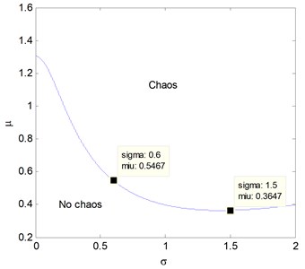
In line with Eq. (13), the chaos boundary for the intensity and the amplitude of bounded noise is given in Fig. 1. It is can be found that there is no chaos under the curve and chaos above it. Moreover, the curve of chaotic boundary declines together with the increase of , which implies the chaos area becomes larger. In the plane, most of the regions are chaotic, and the region with no chaos is very small only when both and are less.
Simultaneously, because that the Melnikov function having the simple zero point is only a necessary condition for the chaos, there is a great difference between the chaotic conditions obtained from the Melnikov method and the numerical results in many problems. In order to verify the validity of Melnikov analytical method in the paper, we select two points 0.6, 0.5467 and 1.5, 0.3647 from the curve to compare the chaos with the numerical safe basins. If the results of analytical method and numerical verification are coincident, the safe basin will be a whole one without erosion in the marked ‘No chaos’ region, but be corroded in the ‘Chaos’ region.
Fig. 1The chaotic boundary in the plane of intensity σ and amplitude μ of the bounded noise a1= 0.345, a3= 1.082, b1= 0.218, b3= 0.672
The numerical simulations are performed in order to prove the analytical prediction of the necessary condition for the chaos. Throughout this paper, the 300 initial values are located in a plane region, i.e., –1.5:0.01:1.5, –1.5:0.01:1.5, and the initial values which make the values of and in the Eq. (5) less than 1.5 after 500 cycles form safe basins. Here, Eq. (5) is solved by the Euler approximation for each initial value. The total time is long enough. In the following numerical calculations, we always assume 0.1.
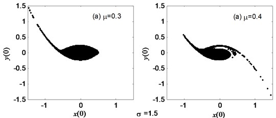
Figs. 2-3 display the erosion of the safe basin with the varied noise amplitude and intensity respectively when other parameters are fixed. It can be found from Fig. 2 that the safe basin is intact at 0.5, 0.6 which shows the chaos does not happen, but the safe basin is damaged at 0.6, 0.6 which illustrate chaos occurs. Moreover, the point 0.5, 0.6 is in the domain of “No chaos” shown in Fig. 1 and the other 0.6, 0.6 is in the area of “Chaos”. The result given in Fig. 3 is the same as the one in Fig. 2: in “No chaos” area, the safe basin is full and broker in “Chaos” region shown in Fig. 1. It illustrates the analytical results obtained by the Melnikov method are well match with the numerical ones gained by the safe basin.
Fig. 2The erosion change of the safe basins with the varied noise amplitude μ as σ= 0.6, a1= 0.345, a3= 1.082, b1= 0.218, b3= 0.672
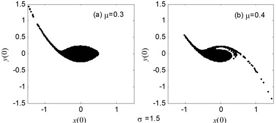
Fig. 3The erosion change of the safe basins with the varied noise amplitude μ as σ= 1.5, a1= 0.345, a3= 1.082, b1= 0.218, b3= 0.672
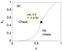
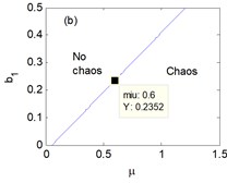
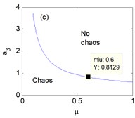
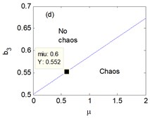
The chaotic regions versus the parameters , , , vary with the increased in Fig. 4 respectively. It can be discovered that the chaotic regions are different and related to the variation of the parameters , , , , , that is, the changes of parameters of the system result in the occurrence of chaos. Moreover, four points are marked as 0.6 in Fig. 4(a)-(d) so as to contrast with the following numerical results.
Fig. 4The chaotic region in the plane: a) μ and a1, b) μ and b1, c) μ and a3, d) μ and b3, at moment σ= 0.6, Y refers to the vertical axis in the plane
4. Parameter-induced erosion of the safe basin
The noise parameters can cause the erosion of the safe basin in Figs. 1-3. However, besides of the perturbations, the variation of other parameters of the system is also an important factor that induces the erosion of safe basin. Therefore, the effects of the linear coefficient, the damping coefficient and the nonlinear coefficient on the erosion of the safe basin are investigated comprehensively in this section. Meanwhile, the analytical chaotic boundaries are verified further.
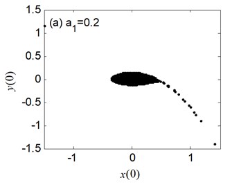
Fig. 5 presents the erosion of safe basin for the different values of linear coefficient of restoring moment . The safe basin is a whole domain of attraction, but very small at 0.2 in Fig. 5(a). During the change process of from 0.8 to 1.6 in Fig. 5(b)-(c), the erosion of the safe basin appears and the area of the safe basin becomes big.
Fig. 5The erosion change of safe basins with the varied a1: μ=σ= 0.6, a3= 1.082, b1= 0.218, b3= 0.672
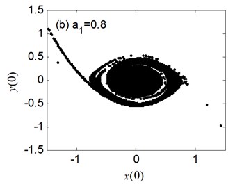
The above results are consistent with the one shown in Fig. 4(a). For the case of 2 in Fig. 6(d), the erosion of the safe basin vanishes and the safe basin is almost filled with the entire plane. Therefore, with the increase of the parameter , the evolution of safe basin will be shown in the “no erosion → erosion → no erosion” form, moreover, the area of safe basin turns larger gradually.
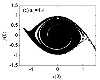
The erosion phenomenon of safe basin versus the linear damping coefficient is put forward in Fig. 6. With the increase of , the safe basin varies from the existence of erosion to no erosion, which is consistent with the chaos region shown in Fig. 4(b). Therefore, it can be found that the increase of linear damping coefficient can strengthen the safe domain of ship navigation.
Fig. 7 shows the erosion of safe basin versus the nonlinear coefficient of restoring moment . The safe basin is an intact domain of attraction for the case of 0.4 and 0.6 in Fig. 7(a)-(b). However, the safe basins are damaged as parameter become bigger in Fig. 8(c)-(d), and the bigger is, the more serious the erosion of safe basin is. Another important result is the area of safe becomes smaller with the increase of . The conclusion in Fig. 7 is generally analogous to the one in Fig. 4(c), but just opposite with the one in Fig. 6.
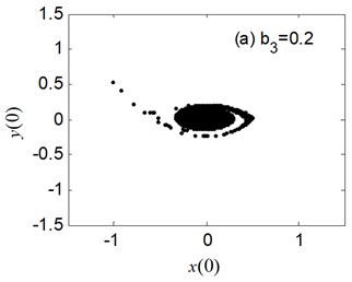
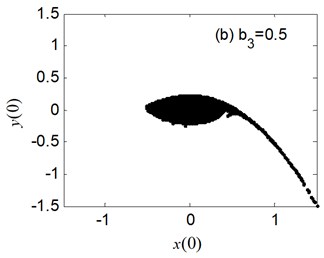
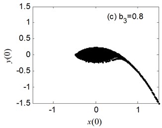
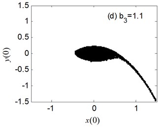
The erosion of safe basin for the different nonlinear damping coefficient is displayed in Fig. 8. We can observe the safe basin is largely eroded at 0.2 in Fig. 8. Then the erosion of safe basin becomes minute little by little with the increase of until erosion disappears at 1.1 in Fig. 8(d).
Fig. 6The erosion change of safe basin with the varied b1: μ=σ= 0.6, a1= 0.345, a3= 1.082, b3= 0.672
Fig. 7The erosion change of safe basin with the varied a3: μ=σ= 0.6, a1= 0.345, b1= 0.218, b3= 0.672
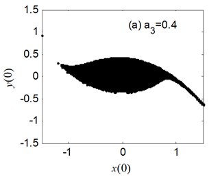
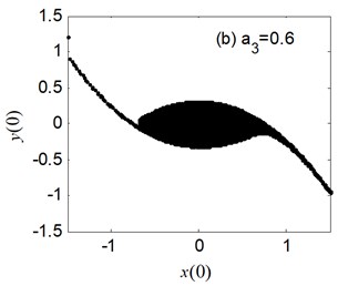
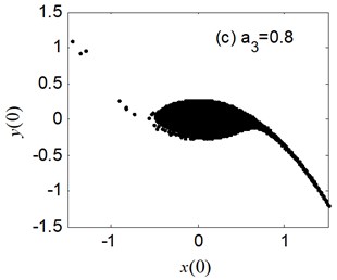
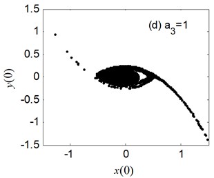
Fig. 8The erosion change of safe basin with the varied b3: μ=σ= 0.6, a1= 0.345, a3= 1.082, b1= 0.218
5. Conclusions
In this paper, the chaos phenomenon of ship rolling motion in stochastic beam seas is investigated. The excitation of stochastic beam seas is regard as a bounded noise which is in good comparison with the P-M spectrum. Thus, the nonlinear model of ship rolling motion is established. In accordance with stochastic Melnikov method, the chaotic threshold about bounded noise parameter is obtained and verified through the numerical safe basin. The numerical results are in good agreement with the analytical predications. Because the non disturbing parameter is also one of the reasons for the erosion of safety basin, the impacts of system parameters on the safe basin are discussed and some interesting phenomena are found. With the increase of linear coefficient of restoring moment , the safe basin varies from no erosion to erosion appearance to no erosion, which implies the evolution of the system is from no chaos to chaos to no chaos. It makes safe basin become complete to increase the damping coefficient , which illustrates the increase of can decrease the chaos and enhance the safety of ship navigation. However, the effect of nonlinear coefficient of restoring moment is opposite with . At last, the increase of nonlinear damping coefficient can also consolidate the safety of ship navigation, which is similar to the effect of .
References
-
Virgin L. N. The nonlinear rolling response of a vessel including chaotic motions leading to capsize in regular seas. Applied Ocean Research, Vol. 9, 1987, p. 331-352.
-
Nayfeh A. H., Khdeir A. A. Nonlinear rolling of ships in regular beam seas. International Shipbuilding Progress, Vol. 33, 1986, p. 40-49.
-
Nayfeh A. H., Khdeir A. A. Nonlinear rolling of biased ships in regular beam seas. International Shipbuilding Progress, Vol. 33, 1986, p. 84-93.
-
Nayfeh A. H., Sanchez N. E. Stability and complicated rolling responses of ships in regular beam seas. International Shipbuilding Progress, Vol. 37, 1990, p. 331-353.
-
Falzarano Shaw S. W., Troesch A. W. Application of global method for analyzing dynamic systems to ship rolling motion and capsizing. International Journal of Bifurcation and Chaos, Vol. 2, 1992, p. 101-105.
-
Bikdash M., Balacpandran B., Nayfeh A. Melnikov analysis for a ship with a general roll-damping model. Nonlinear Dynamics, Vol. 6, 1994, p. 101-124.
-
Liaw Y., Bishop S. R. Nonlinear heave-roll coupling and ship rolling. Nonlinear Dynamics, Vol. 8, 1995, p. 197-211.
-
Tang Y. G., Zheng J. W., Dong Y. Q. Study on the dynamic behavior of the ship’s internal resonance. Shipbuilding of China, Vol. 39, 1998, p. 19-26.
-
Jiang C. B., Troesch A. W., Shaw S. W. Highly nonlinear rolling motion of biased ships in random beam seas. Journal of Ship Research, Vol. 40, 1991, p. 125-135.
-
Hsieh S. R., Troesch A. W., Shaw S. W. A nonlinear probabilistic method for predicting vessel capsizing in random beam seas. Proceedings of the Royal Society of London A, Vol. 446, 1994, p. 195-211.
-
Shen D., Huang X. L. Study on the duration before the ship capsize under the random waves. Shipbuilding of China, Vol. 41, 2000, p. 14-21.
-
Huang X. L., Zhu X. Y. Using path integral method to solve the problem of ship’s capsize probability problem. Journal of Ship Mechanics, Vol. 5, 2001, p. 7-16.
-
Wu W., Mccue L. Application of the extended Melnikov's method for single-degree-of-freedom vessel roll motion. Ocean Engineering, Vol. 35, 2008, p. 1739-1746.
-
Hu K. Y., Ding Y., Wang H. W. Chaotic roll motions of ships in regular longitudinal waves. Journal of Marine Science and Application, Vol. 9, 2010, p. 208-212.
-
Huang X. L. The investigation of the safe basin erosion under the action of random waves. 8th International Conference on the Stability of Ships and Ocean Vehicles, 2003, p. 539-549.
-
Shang H. Control of Erosion of Safe Basins in a Single Degree of Freedom Yaw System of a Ship with a Delayed Position Feedback. Springer, New York, 2010, p. 177-185.
-
Chai W., Fan J., Zhu R. C. The nonlinear ship rolling and safe basins in irregular waves. Journal of Hydrodynamics, Vol. 28, 2013, p. 431-437.
-
Hu K. Y., Ding Y., Wang H. W., Li J. D. Global stability of ship motion in stochastic beam seas. Journal of Harbin Engineering University, Vol. 32, 2011, p. 719-723.
-
Duan F., Xu B. Parameter-induced stochastic resonance and baseband binary pam signals transmission over an AWGN channel. International Journal of Bifurcation and Chaos, Vol. 13, 2011, p. 411-425.
-
Jiang S., Guo F., Zhou Y., Gu T. Parameter-induced stochastic resonance in an over-damped linear system. Physica A, Vol. 375, 2007, p. 483-491.
-
Liu L., Tang Y., Li H. Random jumping of ships with water on deck in beam waves. Ship Building of China, Vol. 50, 2009, p. 1-11.
-
Frey M., Simiu E. Noise-induced chaos and phase space flux. Physica D, Vol. 63, 1993, p. 321-340.
-
Wiggins S. Global Bifurcation and Chaos. Springer, 1998.
-
Simiu E. Melnikov process of stochastically perturbed, slowly varying oscillators: application to a model of wind-driven coastal currents. Journal of Applied Mechanics, Vol. 63, 1996, p. 429-435.
-
Morrall A. The Gaul disaster: an investigation into the loss of a large stern. Naval Architect, Vol. 5, 1981, p. 391-440.
Cited by
About this article

This paper is supported by the National Natural Science Foundation of China (Grant No. 11602098) and the Postdoctoral foundation of Jiangsu Province (Grant No. 1501069B).
