Abstract
Coal mine rescue devices, which can supply miners underground with fundamental shelters after gas explosion, are essential for safety production of coal mines. In this paper, a novel and composite structure-rescue antiknock ball for coal mine rescue is designed. Further, the structural safety and dynamic response under gas explosion of the antiknock ball is investigated by ALE algorithm. To achieve this goal, the ALE finite element method is described in dynamic form, and governing equations and the finite element expressions of the ALE algorithm are derived. 3 balls with different structures are designed and dynamic response analysis has been conducted in a semi-closed tunnel with explosive load of pre-mixed gas/air mixture by using ALE algorithm based on explicit nonlinear dynamic program LS-DYNA. Displacement field, stress field and energy transmission laws are analyzed and compared via theoretical calculations. Results show that the cabin door, emergency door and spherical shell are important components of the rescue ball. The 3# composite ball is the optimization structure that can delay the shock effect of the gas explosion load on a coal mine rescue system; the simulation results can provide reference data for coal mine rescue system design.
1. Introduction
Coal mine accident is impossible to avoid due to the complexity of rock stratum at underground mines. Gas explosion has become one of the most serious disasters for coal mining, the high temperature, high pressure and toxic gases are threatening the underground lives after gas explosion [1]. Therefore, ensuring the health and safety of miners is the prerequisite for safety production. Currently, China, Canada, United States, Chile, South Africa, and Australia have compulsorily demanded that all coal mines must be equipped with rescue equipment including refuge chamber, rescue capsule and any other rescue equipments [2]. Undoubtedly, rescue equipment provides a significant rescue shelter for those who are waiting for rescue, and it has become one of the “six systems” that are provided for coal mine risk prevention [3]. Therefore, study and development for rescue equipment with strong antiknock performance and high temperature resistance is of great significance.
Nowadays, rescue capsule and refuge chamber have become two frequent and important refuge shelters for coal mine emergency rescue during explosion and fire accidents. Meanwhile, numerous researchers [4-10] have conducted many experimental and numerical studies on the antiknock performance of the capsule or chamber. A variety of high-strength, antiknock and high temperature resistant rescue equipment had been designed and developed for safety production of coal mine. Up to now, the rescue capsule and refuge chamber have saved countless lives of miners who had ever trapped in explosion and fire accidents. However, many coal mines have been overwhelmed due to the higher cost, inconvenient movement and bulkiness of refuge chambers and rescue capsule during the great depression of the coal economy. Accordingly, exploiting a novel rescue equipment which is easy to handle and installation with lower cost has become necessary for rescue and safe production of coal mine.
With unique characteristics of soft, low density and buffer ceiling, porous material, especially aluminum foam [11-14] has a better antiknock performance. Consequently, it has attracted a lot of researchers working in the field of explosion engineering. Nevertheless, they are focused on the civil engineering and military equipment. There are seldom research and applications related to gas explosion in coal mines.
In this paper, our purpose is to design and put forward a new type of coal mine rescue ball with special structure based on the new energy absorbing damping material-porous aluminum foam. The nonlinear finite element dynamic analysis method and ALE fluid-solid coupling algorithm are employed to reveal the coupling effect of the gas explosion and structure, and calculate the pressure characteristics, dynamic response and energy variation law in a semi-confined and full-size tunnel. This will provide data basis for structure analysis, development and performance evaluation of coal mine rescue equipments.
2. ALE algorithm and governing equations
2.1. Description for ALE algorithm
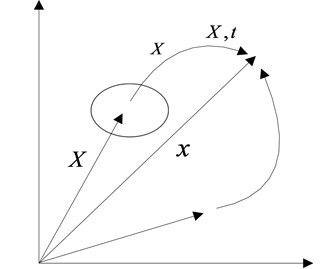
The ALE description for incompressible viscous flows has been developed to solve free surface flows and fluid-structure interaction problems. The configuration of continuum at the initial time is recorded as , and at moment of is . To determine the position of every material point, the Lagrange coordinates (material coordinate) , which is consolidated with objects together and moves along with the object, is established. Then, the position of particle at the initial moment is fully determined by vector . Therefore, could be used to recognize different particles in the interior of an object. The Eulerian coordinates (spatial coordinates) is introduced to describe the current configuration, which is consolidated with space. The position of different points in space is determined by their own location vector in the Euler coordinate system. Thus, can be applied to explain the spatial geometric point.
Lagrange approach describes the motion law of the material point with its initial configuration as the reference configuration in space, which is:
Euler method describes the motion law of the material point with the existing configuration as the reference configuration in space. That is:
The Eq. (1) describes the spatial location of the same particle at different times, and the Eq. (2) describes the same space point occupied by the material points at different moments.
Differences exist between Lagrange and Eulerian descriptions; hence ALE description introduces a new reference configuration that is independent of the initial deformation and the current configurations. The reference configuration is fixed for the observer due to following the reference configuration in the process of deformation of objects, but the initial and current configurations are moving with respect to the reference configuration. Here, a reference coordinate system to determine the corresponding position of each reference point in the reference configuration is introduced. The location of each point in the reference configuration is determined by its location vector in the reference coordinate system, movement rules of material point in the reference coordinate can be expressed as follows:
Nevertheless, the motion law of the reference point in space can be described as follows:
Finite element demonstrated in the material description method is used to split objects, grid point is the material point, that is to say, grid point moves along with the object. Finite element demonstrated in the spatial description method is used to split space, grid points are the spatial points. Therefore, the grid is fixed in space and would not move along with the objects. But the subdivision for finite element mesh aiming at the reference configuration in ALE description method, grid point is reference point, the grid is independent of object and moves along with the space and can be free to choose according to its requirements. The ALE method is described in Fig. 1 [15].
Fig. 1Dynamic description for ALE algorithm
All the mapping described above are one-to-one mapping, both the Jacobi determinant (a description of mapping relationship from the initial configuration to the current configuration) and the mixed Jacobi determinant (a description of mapping relationship from the reference configuration to the current configuration) are not equal to zero, that is:
Assuming that the space point is the image of both a particle and a reference point at the moment , according to the definition that the velocity of a particle is equal to the reciprocal of position vector for time of that particle in the space, which is:
In the reference area, the velocity of a particle in the space, that is to say, the velocity of the grid nodal is equal to the reciprocal of position vector for time of that particle in the space, that is:
In ALE description, the motion law of reference configuration (the computational grid) can be arbitrarily given to a specified motion law of mesh. ALE description can be degenerated into Lagrange description and Eulerian description. When , it means the computational grids are fixed in the space and could be degenerated into Eulerian description. When , it indicates the computational grids move along with the object and degradate into the Lagrange description. When , it describes the independent movement of computational grids in space corresponding to the ecumenical description of ALE.
2.2. Governing equations for ALE algorithm
As for a continuum system, , , are used to reflect the boundaries of the material domain , the spatial domain , and the reference domain , respectively. , , and are the density of the material domain, spatial domain and reference domain, respectively.
The quality of different configurations in the continuum is assumed as . Then, mass conservation equation is:
where, , ,
According to Mass Conservation Law, the overall variance ratio of mass (the reciprocal of matter) should be equal to zero. The equation of mass conservation in the reference domain can be obtained by Eq. (8):
The equation of mass conservation in the spatial domain is:
where, , .
The momentum conservation law shows that the entire variance ratio of the total momentum of the object occupied in reference domain at the moment equals to the sum of the external forces exerted on the object:
where, is the force acting on the surface of the unit of the reference domain and boundary , respectively. is the body force of the unit mass acting on the object.
According to the divergence theorem, the equation of momentum in the reference domain can be deduced as:
where, is the first Piola-Kexihe stress tensor (Lagrange should stress tensor) defined on the reference domain, and its relationship with the Cauchy stress tensor can be described as follows:
It is difficult to work out the Eq. (12) due to the asymmetry of in the reference domain. As the Cauchy stress defined in current configuration is real stress, so it is convenient to transform the certain Eq. (12) into solving the spatial domain in some special cases. Multiplying both sides of the Eq. (12) by , then the following formula can be deduced as follows:
As it can be learnt from the law of conservation of energy, the entire variance ratio of energy (internal energy and kinetic energy) should be the summary of the power that an external force worked on the object and the heat introduced into the object per unit time (other energy, such as electromagnetic energy, and so on, are not in the account). The law of conservation of energy can be expressed as:
where, is energy perunit mass of an object, is the heat flux.
According to the divergence theory, The Eq. (15) the can be turned into a form in reference domain:
where, is energy in unit mass of an object, energy equation in the form of spatial coordinate system is described as following:
2.3. Boundary conditions
In fact, boundary conditions are closely related to the problem that remains to be solved, and has nothing to do with the description method. Therefore, any boundary condition used in the description of Eulerian and Lagrange can be adapted for ALE description. The dynamic boundary is the natural boundary condition, and is automatically satisfied during solution. Here, kinematic boundary conditions used in the Eulerian description are discussed, a complex mathematical mapping needs to be introduced in order to describe moving boundary conditions. Contraried to the Lagrange description, the ALE description is introduced to solve this problem. Therefore, it can be applied on the surface of material by using a Lagrange description, namely:
The formula given above is material surface that satisfies the boundary conditions. When it comes to large deformation flow (such as fluid flow and metal forming and other processing), in order to accurately describe the boundary of an object and maintain a reasonable shape of the grid, generally speaking, such a description is merely used on the surface of the material at normal direction, and allows the grid move along the tangential direction, namely:
where, and refer to the external normal vectors on the surface of the current configuration and the reference configuration. To determine the location of the free surface, the last formula needs to be solved on a free surface. Interface between objections, such as the fluid-structure interaction, contact and friction problems, is another normal boundary condition. In general, two nodes are set up at one point of the interface. Every nod represents one object at one face. These two nodes can move tangentially, bond together, and detach from each other. If two objects are fully bonding together, the corresponding material velocity of the interface nodes should be equal. That is:
If the two objects tangentially slip along the interface, then the corresponding normal material velocity of each node on the interface remains a certain value, namely:
where, is the normal vector of interface, the corresponding material velocity of the interface nodes are independent if two objects separate from each other.
In the ALE formulation, selection of computing grid is independent of the object movement itself. To simplify the process of interface in fluid structure interaction and friction contact, maintaining a coincidence in the deformation process of objects by equaling velocities of the corresponding grid and the other nodes on the interface. This can be described as follows:
Boundary problem is related to the problem to be solved. On the fluid-solid interface of a fluid structure interaction, material boundary condition Eq. (18) is applied to describe the solid interface. Nevertheless, condition Eq. (19) is employed to characterize fluid interface. That is to say, material description should be merely used in the normal direction of the surface in the fluid domain, whereas, motion of tangential grid on the surface has nothing to do with fluid movement, so as to maintain a reasonable shape of the fluid domain mesh.
The steps for ALE calculation are listed as follows:
1) Perform a Lagrange time step, that is, the step only for calculating the effect of the pressure grade distribution on the velocity and the energy change. Since the pressure in the momentum equation is the value of the previous one, it should be in an explicit format.
2) Perform the calculation of the momentum equation, the velocity obtained in the former step would be the first value for iterative calculation.
3) Rezone the mesh and calculate the transport among the meshes.
a) Specify mobile nodes. b) Move the boundary nodes. c) Move the interior nodes. d) Calculate the transport of the element-centered variables. e) Calculate the momentum transport and update the velocity.
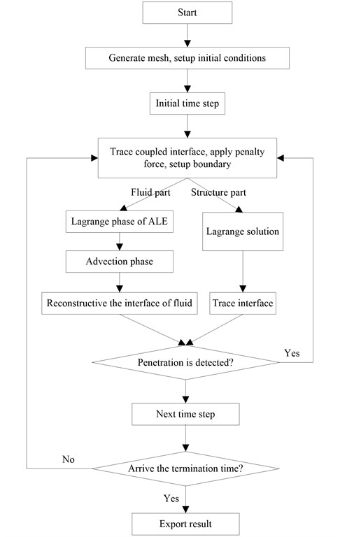
In this article, a penalty-based coupling algorithm in the LS-DYNA ALE package is used. The entire algorithm flowchart is shown in Fig. 2 [16, 17].
Fig. 2Flowchart for ALE algorithm
3. Models and methods
3.1. Geometry and mesh
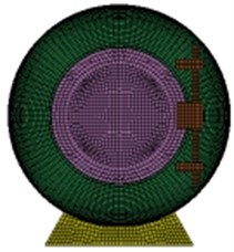
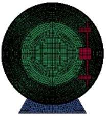
The finite element models of underground rescue ball are established by ANSYS. Solid element is used to express the entity structure such as doors and observation window. And, the shell element is employed to describe the spherical shell. Fig. 3 shows the shape and geometry model of 3 rescue balls with different thickness and materials, of which the cross-section is as large as the inner cross-sectional of the tunnel to prevent and control air leakage. The diameter of the each ball is 1.8 meters. Table 1 lists the material type and thickness of each component on the structure.
Fig. 3The shape and geometry of rescue ball
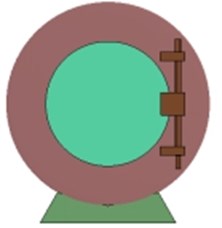
a) 1#
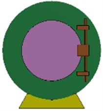
b) 2#
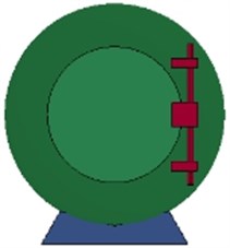
c) 3#
Table 1Material and thickness of each component of the rescue capsule
Component name | Material name | Thickness/mm | ||
1# | 2# | 3# | ||
Cabin door | Q235B/ aluminum foam | 16 S | 16 S | 8 S+5 A+8 S |
Spherical shell | Q235B/ aluminum foam | 8 S | 16 S | 8 S+4 A+8 S |
Emergency door | Q235B/ aluminum foam | 8 S | 8 S | 4 S+3 A+4 S |
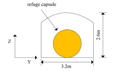
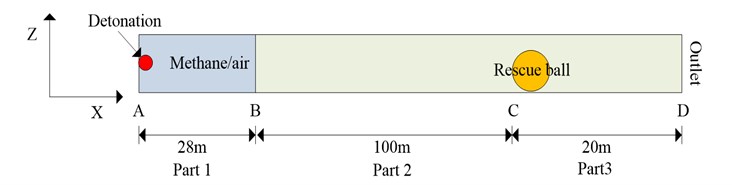
Fig. 4The length and cross-sectional of the tunnel
a) The length of the tunnel
b) The cross-sectional of the tunnel
The simulated tunnel is assumed as a semi-closed pipe model, and the corresponding size is illustrated in Fig. 4. As it can be seen from the figure, the tunnel is divided into 3 parts and its total length is 148 m. Part 1 (from A to B) the explosion source, a length 28 m of methane/ air mixture, which is full of 200 m3 methane/air mixture with 9.5 % concentration. Part 2 (from B to C) air transmission section, a length of 100 m air zone. Part 3 (from C to D) starts from the impact face of the rescue ball and ends in the exit of the tunnel, which is 20 meters long. The bottom bracket of rescue ball is fastened to the ground. Assume that the initial velocity of rescue ball is zero, and the roof, ground, wall of the tunnel is smooth and rigid. Regardless of the energy absorbed by the roof, ground and wall of the tunnel are not into account.
Taking into account the actual size of the established model above, the shell element is divided with tetrahedral element mesh and the rescue ball is meshed with the mapping method. Shell 163 element is employed to simulate, the size of each unit is 0.04 m. The cabin door, emergency door, spherical shell and methane/air mixture, and air section are meshed with hexahedral grid and simulated with 164 elements, the element size of fluid and solid is 0.1 m. Grid of each ball is illustrated in Fig. 5, respectively.
The coupling algorithm is adopted to simulate the interaction between fluid and structure. ALE method is employed to divide the fluid domain, while Lagrange deformable mesh is used for partition of the solid domain. The coupling force of interface of fluid-structure is calculated via ALE coupling algorithm. These forces are added to the nodal forces of fluid and the structure by explicit finite element method simulation. It is necessary to choose an accurate fluid-structure coupling algorithm to predict local peak pressure of the structure. This paper presents a penalty contact function which is similar to the analysis of Euler and Lagrange coupling algorithm.
Fig. 5The mesh of geometrical model
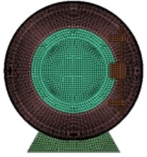
a) 1#
b) 2#
c) 3#
3.2. Material models and state equation
The main component of the mixture is methane. It has been proved that if the concentration of methane ranges from 5 % to 15 % in the premixed gases, a minimal energy will easily trigger a gas explosion. The explosion speed and pressure of methane/air mixture can reach the maximum when the methane concentration reaches about 9.5 % [18, 19].
The air and gas flow state are described by material MAT_NULL model in the material database of LS/DYNA and the linear polynomial equation of state EOS_LINEAR_POLYNOMIAL. The linear polynomial equation of state is expressed as follows:
where, is the initial density, is the current density, is the internal energy. - are state parameters of the Eq. (23), .
The parameter values of null material model and linear polynomial equation of state are shown in Table 2.
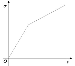
The process of impact and dynamic under gas explosion is a typical high-strain-rate phenomenon. The mechanical properties of steel will change noticeably when affected by the rate of explosive load. The yield strength of the material will increase substantially under high strain rate [20]. In this paper, the nonlinear plastic material model PLASTIC-KINEMATIC proposed by Symonds and Cowper [21] is employed to simulate the strain rate effect of steel, the Constitutive curve of the model is described in Fig. 6(a):
where and are the stress and strain of the material, respectively and are Cowper-Symonds constants, the suggested values for steel are 40.4 and 5, respectively. is hardening parameter, which means that kinematic hardening if 0 but isotropic hardening if 1. is the initial yield stress, is the strain rate, is the effective plastic strain, is the yield strength, is the plastic hardening modulus and determined by the following calculation:
where, is the Yield hardening modulus, is the Elastic modulus. The nonlinear plastic material model plastic kinematic is applicable for metal materials under blast loading. The calculated results are in good agreement with the experimental data. The mechanical properties of material parameters are shown in Table 3.
Table 2Parameters used in linear polynomial equation of state.
Material | Density (kg/m3) | (Pa) | E (J/m3) | |||||||
Air | 1.29 | –1×10⁵ | 0 | 0 | 0 | 0.4 | 0.4 | 0 | 2.5×10⁵ | 1 |
Methane/air mixture | 1.23 | 0 | 0 | 0 | 0 | 0.274 | 0.274 | 0 | 3.4×10⁵ | 1 |
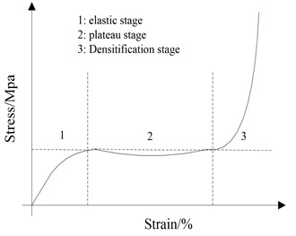
Fig. 6Constitutive curves for steel and aluminum foam. a) Elastic-plastic constitutive model, b) Constitutive curve of aluminum foam
a)
b)
Table 3Parameters used in state equation of steel
Steel | Yield strength / MPa | Hardening modulus / MPa | Elastic modulus/ GPa | Poisson’s ratio | Failure strain / | |||
Q235B | 235 | 1050 | 208 | 0.3 | 5 | 5.0 | 0 | 0.35 |
The constitutive curve of aluminum foam under quasi-static loading is shown in Fig. 6(b). As it can be seen, this curve has three stages, which are elastic stage, ideal plastic / softening stage, and rapid densification stage. In the first stage, deformation mainly occurred on the skeleton part of aluminum foam due to external pressure and elastic deformation. In the second stage, the skeleton part is prone to broken when the external pressure exceeds the yield strength. Then, the strain is rapidly increased. Nevertheless, stress increases a little because of skeleton broken. In the third stage, changes of both stress and strain are liner because the broken skeleton compressed together and solidifies into foam.
Kinslow R. [22] put forward a one-dimensional model to describe the stress-strain relationship of polymer foams:
where, , are Hugoniot parameters, is Grueisen coefficient, is specific heat inconstant volume, is coefficient of linear expansion. The parameters in the Eq. (26) are given in Table 4.
Table 4Parameters used in equation of state for Crushable foam
/ kg·m3 | / km·s-1 | / MPa | / MPa | Poisson’s ratio | Elastic modulus / MPa | ||
480 | 0.52 | 51 | 6.5 | 0.31 | 42 | 1.26 | 1.51 |
3.3. Simulation assumptions
Further hypothesizes are needed to be made in order to eliminate the impact of unfavorable factors:
A. Air is non-viscous ideal gas, and the process of the shock wave expansion is an equal-entropy and adiabatic.
B. Regardless of the change of the material properties and the influence of the welding angle on the structure.
C. Material is homogeneous and isotropic.
D. Deformation caused by production and installation can be ignored, there is no relative movement between different components.
E. The bolt connection is reliable, and the pre-stress has no effect on the entire structure [23].
F. Ignoring the influence of high temperature on the material properties.
4. Validation for gas/air mixture explosion in a semi-closed tunnel
4.1. Reflection of shock waves in solid surface
When the shock wave encountered with obstacles in the tunnel, the peak pressure and velocity of shock wave will increase rapidly around the obstacle due to the incentive effect [24]. According to the theory of shock wave, shock wave will transmit and reflect simultaneously at the interface when the shock wave arrives at the solid surface. If the impedance of the shock wave is greater than that of the incident wave, the pressure of the reflected shock wave will increase substantially. According to the continuity condition of the interface, the pressure and particle velocity on both sides should satisfy the following relationships:
The velocity of particles on the solid surface can be defined according to one-dimensional driven theory as follows:
The equation of state of solids is expressed as follows:
where, is the pressure of the incident wave, is the pressure of the reflected wave. is the velocity of the incident wave. is adiabatic coefficient of gas. is an engineering constant. is the velocity of particle on the interface. The Eqs. (30-31) are transcendental equations both related to . The approximate solution of can be obtained by using Newton iterative method.
4.2. Validation of blast model
To investigate the dynamic response under gas explosion load, shock wave attenuation law of gas explosion is the premise. In order to obtain the real peak pressure of overpressure of blast wave at different measuring points along a tunnel, Bjerketvedt [24] carried out a large scale gas explosion experiment with 9.5 % methane/air concentration premixed mixture whose volume is 200 m3. Tian [25] has theoretically deduced the non-linear relationship between gas explosion overpressure and distance, the cross-sectional area of the tunnel and methane volume (initial explosion energy). Normally, the following Eq. (32) is used for calculating the explosion overpressure:
where, is air density, is local velocity of sound, is adiabatic compression coefficient, is the distance between explosive center and the front of shock wave, is the cross-sectional area of the tunnel, is the total energy released by gas explosion [25].
Fig. 7Comparison of the experimental, theoretical and numerical data in 200 m3 methane explosion

In general, the theoretical calculation results are slightly larger than the experimental data due to a few ideal hypotheses for the theoretical analysis. However, accumulation of energy is in accordance with the mechanism of chemical reaction dynamics in real explosion conditions. Therefore, the explosion overpressure increases to a maximum and decrease thereafter. In order to ensure the simulated results and the experimental data are in a good accordance, the energy factor is introduced. Thus, the pressure of the gas explosion is obtained as follows [26]:
where, can be obtained through data fitting, and the expression is described as follows:
The experimental data [27], theoretical data [28], the modified data [29], and numerical data [30] about the peak value of overpressure versus the distances are displayed in Fig. 7. As it can be seen, the numerical simulation data are in agreement with the experimental data and the theoretical value. The numerical simulation results are higher than the theoretical value and the experimental value because the wall of the tunnel is rough and can absorb energy.
Fig. 8Pressure contour of the blast wave interact with the rescue ball in the tunnel
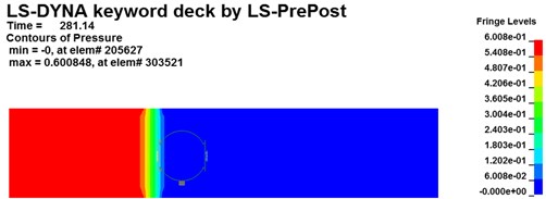
a)281.14 ms
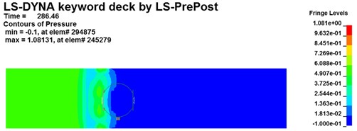
b)286.46 ms
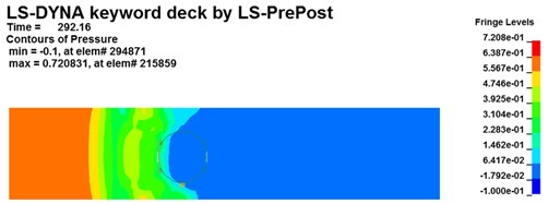
c)292.16 ms
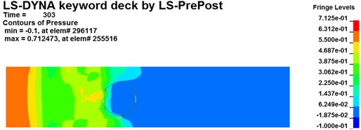
d)303 ms
5. Results and discussions
5.1. Fluid-structure interaction effect
Pressure contours for shock wave interact with the coal mine recue ball at different moments are shown in Fig. 8 (Taking 1# ball as an example). As it can be noticeable found that the flow field of gas explosion affect and restrict with the capsule. The explosion products generated and expended quickly from one end of the tunnel across the surface of the ball. The shock wave disordered in the initial stage, and the chaotic flow field begins to stable with the propagation of shock wave and formed the plane shock wave in the end. Before the shock wave meets and contacts the ball, the peak pressure of the incident wave is about 0.36 MPa at 281 ms (see in Fig. 8(a)). However, the peak pressure of the incident wave at 286 ms increased to 0.72 MPa as the shock wave contacts the ball. This is mainly because that a velocity gradient field formed around the chamber resulted from the combined action of the shock wave and the reflective wave. The peak pressure of the incident wave quickly decreases due to the energy absorption by coal mine mobile rescue ball and multiple reflections and diffractions. The peak pressure in the tunnel decreases sharply to 0.38 MPa at 303 ms, while the pressure on ball gradually decays and approaches to a nearly constant value of 0.14 MPa (see in Fig. 8(d)). Therefore, the ALE fluid-structure coupling method can be more intuitive to reveal the complex interaction of between gas explosion shock wave and rescue ball in underground tunnels.
5.2. Dynamic response of rescue ball
5.2.1. Stress field
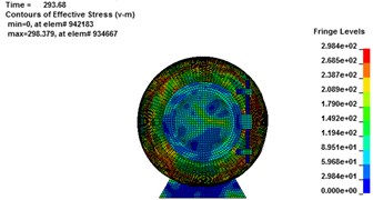
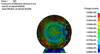
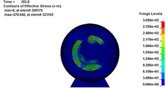
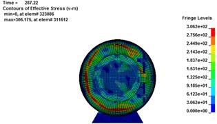
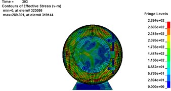
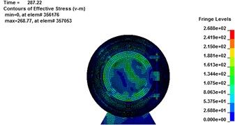
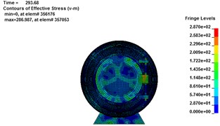
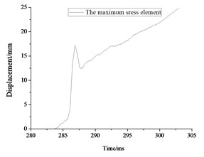
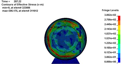
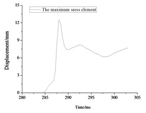
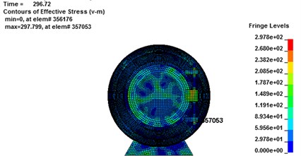
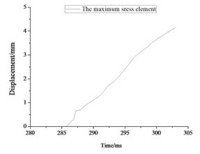
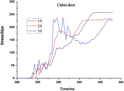
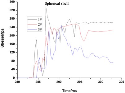
The stress contours of the rescue balls at different moments show in Fig. 9, which indicates that the pressure is gradually increased from blue to red. Table 5 lists the stress results of cabin door, emergency door, and spherical shell. For the 1#, 2# and 3# rescue ball, the equivalent stress of the cabin door increases gradually as the shock wave propagates. The shock wave spreads to the surface of the ball and begins to exert pressure on the ball at the moment of 283.8 ms. Higher stress appears at the spherical shell while lower stress on the cabin door and emergency door of the ball during the entire process. Stress concentration appears at the cabin door and impact face of spherical shell. The maximum stress concentration appears at top, bottom and intermediate surface of spherical shell. As it can be seen from Fig. 10(a), the stress of elements 9422183 (1#), 311612 (2#) and 357053 (3#) reaches the maximum, respectively at the moments of 286 ms, 287.2 ms and 296.7 ms, respectively. The maximum absolute displacements of those 3 elements are about 25 mm, 12.4 mm and 4.2 mm at the moment of 303 ms, as shown in Fig. 10(b). No obvious plastic deformation appears and the stress of elements at the other portions of the 3# ball does not exceed the material yield strength. When the peak overpressure of gas explosion reaches about 0.71 MPa, the strength of the overall structure and main parts are in the elastic range. Because of the short time of explosive shock, stress concentration and plastic zone do not lead to the failure of the entire ball.
Table 5Numerical simulation results for stress on rescue ball
Components of the structure | The element maximum stress / MPa | Time of occurrence / ms | The maximum stress concentration area of the rescue ball | ||||||
1# | 2# | 3# | 1# | 2# | 3# | 1# | 2# | 3# | |
Cabin door | 259.2 | 228.9 | 232.6 | 303 | 303 | 303 | On edge of cabin door | On edge of cabin door | On edge of cabin door |
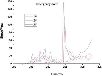
Emergency door | 58.7 | 165 | 214.8 | 303 | 303 | 295.9 | On edge of emergency door | On central of emergency door | On central of emergency door |
spherical shell | 159.2 | 119.7 | 39.6 | 294.7 | 295 | 286.8 | On impact face of spherical shell | On impact face of spherical shell | On impact face of spherical shell |
Fig. 9Von Mises stress cloud chart for rescue balls. (a-d), (e-h) and (i-l) are Von Mises stress cloud chart for 1#, 2# and 3# rescue ball, respectively
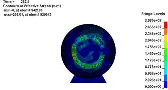
a)283.8 ms

b)287.22 ms
c)293.68 ms
d)304.4 ms
e)283.8 ms
f)287.22 ms
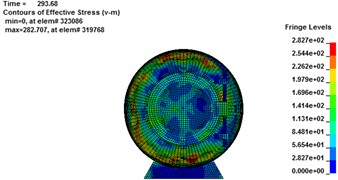
g)293.68 ms
h)304.4 ms
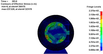
i)283.8 ms
j)287.22 ms
k)293.68 ms
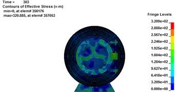
l)304.4 ms
Fig. 10Maximum stress result for rescue ball. (a, c, e) stress cloud chart for maximum stress element, (b, d, f) the maximum stress element time history
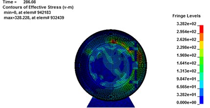
a)
b)
c)
d)
e)
f)
5.2.2. Displacement field
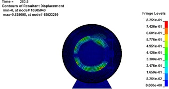
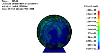
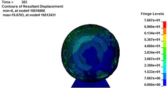
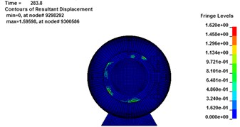
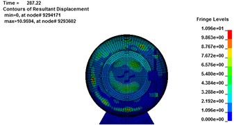
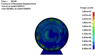
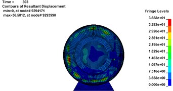
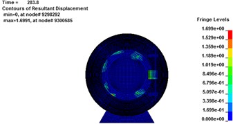
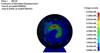
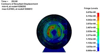
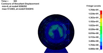
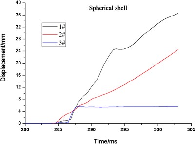
Fig. 11 shows the displacement contour of the 3 balls at different moments. The transition of the color from blue to red indicates that the displacement changes from small to large. Table 6 lists the displacement results of cabin door, emergency door, and spherical shell. Deformation on the cabin door and impact face of spherical shell is most obvious due to the first impact of the explosion shock wave. As the shock wave gradually propagates forward and be reflected by the tunnel wall, displacement of those 3 balls increases because superimposed deformation and continuous force exerted by explosion blast wave.
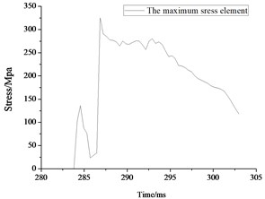
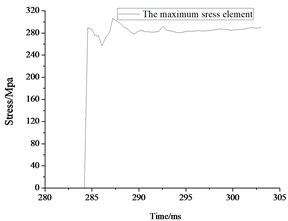
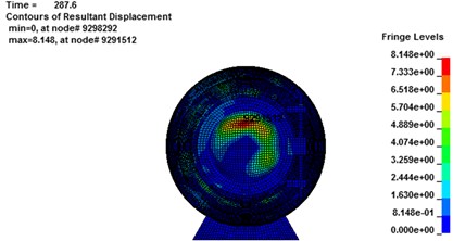
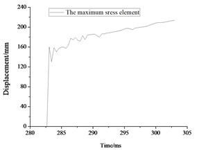
As it can be seen from Fig. 11, the largest deformation emerges in the impact surface of the spherical shell. So the spherical shell requires the best tightness to prevent carbon monoxide and other poisonous gases generated by gas explosion. As Fig. 12(a) shows, the displacement of nodes 18517034 (1#), 9293990 (2#) and 9291512 (3#) reaches the maximum at 292.5 ms, 303 ms and 287.7 ms, respectively. The maximum absolute stress of those 3 nodes are about 328 MPa, 306 MPa and 232 MPa at the moment of 287 ms, 285.6 ms and 303 ms, respectively, as shown in Fig. 12(b). However, the absolute maximum displacement of 1# and 2# balls has exceeded 20 mm and could not guarantee the safety of the rescue according to code for design of mine rescue equipment. For the 3# rescue ball, there is no local brittle fracture and crack, meaning that the safety of the cabin door and spherical shell meets the safety requirements.
Fig. 11Displacement change for rescue ball. (a-d), (e-h) and (i-l) are displacement change cloud chart for 1#, 2# and 3# rescue ball, respectively
a)283.8 ms

b)287.22 ms
c)293.68 ms
d)304.4 ms
e)283.8 ms
f)287.22 ms
g)293.68 ms
h)304.4 ms
i)283.8 ms
j)287.22 ms
k)293.68 ms
l)304.4 ms
Table 6Numerical simulation results for displacement on rescue ball
Components of the structure | The maximum displacement / MPa | Time of occurrence / ms | The maximum displacement concentration area of the rescue ball | ||||||
1# | 2# | 3# | 1# | 2# | 3# | 1# | 2# | 3# | |
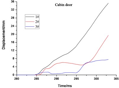
Cabin door | 34.9 | 18.2 | 6.2 | 303 | 303 | 303 | On edge of the cabin door | On edge of cabin door | On edge of cabin door |
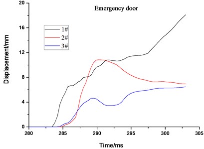
Emergency door | 18.4 | 10.9 | 6.1 | 303 | 290 | 303 | On edge of emergency door | On central of emergency door | On central of emergency door |
spherical shell | 36.2 | 23.1 | 5.8 | 303 | 303 | 287.2 | On impact face of spherical shell | On impact face of spherical shell | On impact face of spherical shell |
Fig. 12Maximum displacement result for rescue ball. (a, c, e) displacement cloud chart for maximum displacement element, (b, d, f) the maximum displacement element time history

a)
b)

c)
d)
e)
f)
The stress and displacement-time curves of the maximum element of the cabin door, emergency door, and spherical shell show in Fig. 13, respectively. Impacted by the gas explosion, the dynamic response of the impact face is the most violent, leading to the maximum of equivalent stress and displacement larger than those of other face and components. The stress and displacement of the escape door is relatively smaller due to the weaker dynamic response. All the residual displacements on the rescue ball are less than 8mm for the 3# ball (see in Fig. 13(b)). As discussed above, the 3# rescue ball has a better antiknock performance under the 200m3 gas explosion shock load [23].
Fig. 13The maximum stress and displacement element time history for cabin door, emergency door, spherical shell
5.3. Energy transmission law
Fig. 14 shows the variation law of internal energy, kinetic energy, and the total energy of ball interact with flow field of gas explosion. Internal energy consists of elastic strain energy, pseudo strain energy, and energy dissipation in the viscoelastic and creep process. As can be seen from the Fig. 14(a), internal energy and kinetic energy change on the contrary law, the difference, including energy dissipation and pseudo strain energy, between the two in numerical is about 1 order of magnitude. The kinetic energy increases firstly until maximum and then decreases sharply with the propagation of shock wave thereafter and tends to balance eventually. As can be seen in the Fig. 14(b), the 2# and 3# rescue ball can absorb energy and thus decrease the harm caused by gas explosion shock wave. The 3# ball could better absorb and store energy effectively by using the intermediate medium of aluminum foam. When the ball is completely submerged by the shock wave, the ball is still in static state, the kinetic energy reaches the minimum while internal energy attains the maximum.
Fig. 14Energy variation law of the structure under explosion load
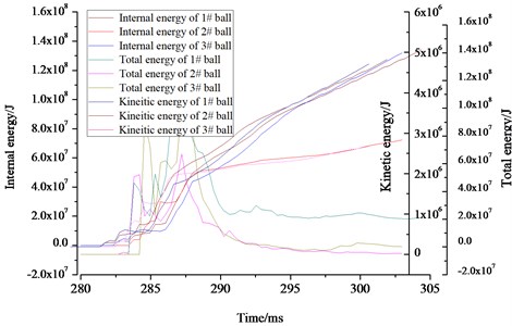
a) The variation law of internal energy, kinetic energy and total energy for 3 balls
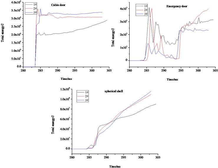
b) The variation law of total energy for cabin door, emergency door and spherical shell of 3 balls
6. Conclusions
In this paper, the nonlinear dynamic finite element analysis software ANSYS/LS-DYNA was applied to investigate structural safety and dynamic response of 3 different coal mine rescue balls under 200m3 air/gas mixture explosion blast based on ALE algorithm. The following conclusions can be drawn:
1) The ALE finite element method is described in a dynamic form. Further, governing equations and the finite element expressions of the ALE algorithm are derived. The simulation method for antiknock performance of structure with gas explosion blast load was proposed based on ALE algorithm. The ALE algorithm can be applied to the field of gas explosion shock and large deformation of structures.
2) The influence of the ball on the shock wave advance is pronounced. The shock wave is reflected by the ball and the reflected wave pressure on the impact surface is about two times higher than that on the incident wave pressure. The antiknock performance of 3 different rescue balls with gas explosion blast for given conditions was simulated by ANSYS/LS-DYNA software. And, pressure in the tunnel conformed well to the reported data.
3) During the interaction process of gas explosion shock wave and rescue balls, the maximum equivalent stress and the absolute maximum displacement concentrate locate at the impact face of spherical shell and the edge of the impact face, respectively. The entire 3# ball is in elastic state without other plastic deformation, the strength can satisfy the safety requirements and standards.
4) Kinetic energy and internal energy of the rescue ball follow certain rules, but change tendency of them were opposite. The kinetic energy reaches to the maximum in situ where the shock wave contact with the rescue ball. Kinetic energy decreases with the propagation of shock wave. When the ball was completely submerged into the shock wave, the 3# ball is still in static state. Then, the kinetic energy reaches the minimum while internal energy attains the maximum.
References
-
Wang K., Jiang S. H., Ma X. P., Wu Z. Y., et al. Study of the destruction of ventilation systems in coal mines due to gas explosions. Powder Technology, Vol. 286, 2015, p. 401-411.
-
Mine Safety and Health Administration. Federal Register, Department of Labor, Vol. 73, Issue 25, 2008, p. 656-700.
-
Niu H. Y., Deng J., Zhou X. Q., Wang H. Q. association analysis of emergency rescue and accident prevention in coal mine. Procedia Engineering, Vol. 43, 2012, p. 71-75.
-
Margolis K. A., Westerman C. Y., Kowalski-Trakofler K. M., et al. Underground mine refuge chamber expectations training: program development and evaluation. Safety Science, Vol. 49, 2011, p. 522-530.
-
Mitchell M. D. Analysis of Underground Coal Mine Refuge Shelters. Doctoral Dissertation. West Virginia University, 2008.
-
Fan X. T. Study on blast performance of refuge chamber. Mining Safety and Environmental Protection, Vol. 37, Issue 3, 2010, p. 25-30.
-
Zhao H., Qian X. M., Li J. Simulation analysis on structure safety of coal mine mobile refuge chamber under explosion load. Safety Science, Vol. 50, Issue 4, 2012, p. 674-678.
-
Zhang B. Y., Zhao W., Wan W., Zhang X. H. Pressure characteristics and dynamic response of coal mine refuge chamber with underground gas explosion. Journal of Loss Prevention in the Process Industries, Vol. 30, 2014, p. 37-46.
-
Mei R. B., Li C. S., Cai B., Liu X. H. FEM analysis of anti-deformation capability for coal mine refuge chamber suffered to gas explosion. Journal of Northeastern University, Vol. 34, Issue 1, 2013, p. 85-94.
-
Song M., Ge S. R. Dynamic response of composite shell under axial explosion impact load in tunnel. Thin-Walled Structures, Vol. 67, 2013, p. 49-62.
-
Rizov V. I. Low velocity localized impact study of cellular foams. Materials and Design, Vol. 28, Issue 10, 2007, p. 2632-2640.
-
Ajendran R., Moorthi A., Basu S. Numerical simulation of drop weight impact behavior of closed cell aluminum foam. Materials and Design, Vol. 30, Issue 8, 2009, p. 2823-2830.
-
Ruan D., Lu G., Wong Y. C. Quasi-static indentation tests on aluminum foam sandwich panels. Composite Structures, Vol. 92, Issue 9, 2010, p. 2039-2046.
-
Yu J., Wang E., Li J., et al. Static and low velocity impact behavior of sandwich beams with closed cell aluminum foam core in three-point bending. International Journal of Impact Engineering, Vol. 35, Issue 8, 2008, p. 885-894.
-
Souli M., Shahrour I. Arbitrary Lagrange Eulerian function for soil structure interaction problems. Soil Dynamics and Earthquake Engineering, Vol. 3, 2011, p. 72-79.
-
Ls-Dyna Keyword User’s Manual (Version 971). Livermore Software Technology Corporation, California, US, 2011.
-
Ahmadi K., Aquelet N. Delayed mesh relaxation for multi-material ALE function. International Journal of Heat and Fluid F1ow, Vol. 46, 2014, p. 102-111.
-
Lee J. H. Overview of gas explosions and recent results in the study of turbulent de deflagrations and detonations. Proceedings of Conference on the Control and Prevention of Gas Explosions, London, 1983, p. 33-36.
-
Lee J. H. Explosion in vessels: recent results. New data on explosions in closed and vented vessels provide valuable tools for loss-prevention engineers. Plant/Operations Progress, Vol. 2, Issue 2, 1983, p. 84-89.
-
Liew Richard J. Y. Survivability of steel frame structures subject to blast and fire. Journal of Constructional Steel Research, Vol. 64, 2008, p. 854-866.
-
Cowper G. R., Symonds P. S. Strain-Hardening and Strain-Rate Effects in the Impact Loading of Cantilever Beams (No. TR C 11 28). Brown University of Providence RI, United States, 1957.
-
Kinslow R. High-Velocity Impact Phenomena. Academic Press, New York, 1970.
-
AQ2011-11-3 Simulation and Analysis of Standard Numerical Shock Resistance of Explosion of Coal Mine Underground Movable Lifesaving Cabin. State Administration of Work Safety, 2011.
-
Bjerketvedt D., Bakke J. R., Van Wingerden K. Gas explosion handbook. Journal of Hazardous Materials, Vol. 52, Issue 1, 1997, p. 1-150.
-
Tian Z. M., Wu Y. B., Luo Q. F. Characteristics of in-tunnel explosion induced air shock wave and distribution law of reflected shock wave load. Journal of Vibration and Shock, Vol. 30, Issue 1, 2001, p. 21-26.
-
Wang H. Y., Cao T., Zhou X. Q., et al. Research and application of attenuation law about gas explosion shock wave in coal mine. Journal of the China Coal Society, Vol. 34, Issue 6, 2009, p. 778-782.
-
Wu B. Study on the Thermal Dynamics of Premixed Methane-Air Deflagration Process in Half-Confined Space in Coal Mine. Dissertation, China University of Mining and Technology, 2003.
-
Qu Z. M., Zhou X. Q., Wang H. Y. Overpressure attenuation of shock wave during gas explosion. Journal of China Coal Society, Vol. 33, Issue 4, 2008, p. 410-414.
-
Xu L. Study on the Attenuation Law and Safe Distance of Gas Explosion Shock Wave. Master Thesis. China University of Mining and Technology, 2015.
-
Zhang B. Y., Zhao W., Wan W., Zhang X. H. Pressure characteristics and dynamic response of coal mine refuge chamber with underground gas explosion. Journal of Loss Prevention in the Process Industries, Vol. 30, 2014, p. 37-46.
About this article

National Key Research and Development Plan (Grant No. 2016YFC0800102), National Natural Science Foundation (Grant No. 51504190 and No. 51604218), General program of National Natural Science Foundation (Grant No. 51674191 and No. 51674192), Scientific Research Program Funded by Shaanxi Provincial Education Department (Grant No. 2013JK0947), Postdoctoral Science Foundation of China (Grant No. 2013M530430), International Science and Technology Cooperation and Exchange of Shaanxi Province (Grant No. 2016KW-070), Postdoctoral Science Foundation of Xi’an University of Science and Technology (Grant No. 2016QDJ013 and No. 2015T81043).
Xiaokun Chen put forward the theme and idea of this manuscript. Haitao Li conducted the simulation and wrote this manuscript. Yutao Zhang revised the grammar of this manuscript. Qiuhong Wang edited the format of this manuscript. Yongfei Jin presented a novel design for recue ball simulated in this manuscript.
