Abstract
Rolling mill is the core equipment in modern iron and steel industry, and the reliability of its mill roll system (MRS) is the key to ensure the rolling process with high precision, high speed, continuity and stability. However, the MRS possesses some features such as high nonlinearity, time variability and strong coupling. The vertical vibration easily happens in its working process. Nevertheless, the mathematical model of MRS is difficult to be established and hard to be solved. In this paper, the nonlinear dynamics theory and modern signal processing method were introduced to solve this difficult problem. A two degree of freedom (DOF) nonlinear vertical vibration model of MRS was established. And the model was analytically solved by using complexification averaging (CA) method. The solution error of CA method was thoroughly analyzed. Moreover, the CA method was improved by combining the fast empirical mode decomposition (FEMD) method. Research results indicate that the improved CA method presents a significant advantage in improving the solution precision, and can be used to solve strong nonlinear vibration system (NVS) with two DOF.
1. Introduction
Rolling is a metal forming process in which a metal strip is laminated through a pair of rolls. In modern iron and steel industry, rolling mill is the core equipment in rolling process. And the operational reliability of MRS is the key to guarantee the rolling process with high precision, high speed, continuity and stability [1]. In steady rolling process, the force balance relation will be destroyed when MRS is disturbed by interference force, and the vertical vibration will be produced [2, 3]. The vertical vibration of MRS has a significant effect on rolling precision and product quality. So, the vertical vibration of MRS is worthy of attention. In addition, MRS is a complex dynamics system composed of many parts. It possesses some special characteristics such as high nonlinearity, time-variability and strong coupling. Hence, it is difficult to precisely establish a mathematical model [4]. At present, the nonlinear factors are not taken into consideration in most of modeling, or linearized by the small deviation theory. The linearized model is frequently used to replace the actual nonlinear system [5, 6]. In sometimes, however, it will cause a large error if some small nonlinear factors are ignored in the actual calculation and analysis. With the development of nonlinear science, researchers pay high attention to nonlinear factors, and begin to explore in this field [7, 8]. Therefore, it is worth further research about introducing the nonlinear dynamics theory and method for the modeling of MRS.
The traditional quantitative analysis methods for nonlinear system mainly include Lindstedt-Poincaré method [9], multi-scale method [10], average method [11] and KBM method [12]. The common point of these methods is to treat the nonlinear factors as a small perturbation attached to linear system [13]. These traditional analysis methods require that the nonlinear terms must be very small. They only apply to solve the weak NVS [14, 15]. In 1999, the complex-variable quantization thought was applied to nonlinear coupling vibration by Manevitch L. I. [16]. And a method named complexification averaging (CA) was proposed, which was gradually evolved into a kind of analytical method for NVS. The CA method is not limited to weak NVS. It not only can be utilized to solve the system with strong nonlinear terms, but also can be used to solve the system with multiple degree of freedom (MDOF) [17]. However, the CA method still has some errors when it is used to solve the strong NVS with MDOF. Therefore, the solution accuracy still needs to be further improved.
In recent years, an adaptive signal processing method named empirical mode decomposition (EMD) was proposed by professor Huang etc. [18]. The method changed the helpless predicament for dealing with nonlinear and non-stationary signal. It can decompose the non-stationary signal into a set of steady data series. So, it has aroused great attention in the international academic circles. Since EMD was put forward, it has been applied to many researches such as physics [19], biomedicine [20], machinery fault diagnosis [21], image analysis [22], pattern recognition [23] and so on. A series of valuable research results were obtained. However, in the process of researches, it was found that although EMD was very suitable for processing non-stationary signal, the mode mixing phenomenon exists [24]. In order to overcome the defects of EMD, a novel method called fast empirical mode decomposition (FEMD) was put forward by professor Wang etc. [25]. And it was proved that FEMD could significantly improve computation speed and effectively restrain mode mixing.
In this work, we attempt to utilize the nonlinear dynamics theory and modern signal processing method to explore the analytical solution for nonlinear vertical vibration model of MRS. In Section 2, the nonlinear vertical vibration model of MRS is established. In Section 3, the model is analytically solved by CA method. In Section 4, in order to improve the solution accuracy, an improved CA method is proposed by combining FEMD method, so that the improved CA method can be used to solve strong NVS. Finally, some conclusions are provided in Section 5.
2. Nonlinear vertical vibration model of mill roll system
MRS is a distributed mass system with MDOF. So, the analysis for the system are very complicated. At present, in order to facilitate the analysis, MRS is mainly divided into two load models: the lumped load model with single DOF and the distributed load model with MDOF. Moreover, researches show that the performance of the asymmetric distribution model with two DOF more correspond with the actual working condition [26, 27].
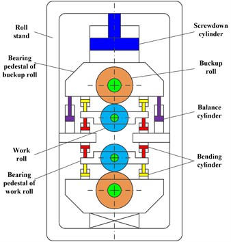
In this paper, the four rollers mill is employed as a research object, and the distributed mass model with two DOF is adopted as foundation. Then, the upper backup roll and work roll are seen as a mass system, and the lower backup roll and work roll are served as another mass system. Moreover, the nonlinear elastic force and nonlinear damping force are considered. The structural form of Duffing oscillator and Van der pol oscillator are respectively defined as the nonlinear stiffness term and nonlinear damping term [28, 29]. Furthermore, a nonlinear vertical vibration model of MRS is established, as shown in Fig. 1.
The dynamic equilibrium equation of MRS at vertical vibration can be expressed by:
where and are the equivalent quality of moving parts of the upper roll system (URS) and lower roll system (LRS); and are the linear damping coefficient (DC) of moving parts of the URS and LRS; and are the nonlinear DC; and are the linear stiffness coefficient (SC) between the frame beam and the moving parts of URS or LRS; and are the nonlinear SC; is the DC between work roll and rolled piece; is the SC between work roll and rolled piece; and are the vibration displacement of the URS and LRS.
Fig. 1Structure of four rollers mill and its nonlinear mechanics model
3. Solve the model of mill roll system based on CA method
3.1. Basic principle of CA method
In 1999, a pair of conjugate complex variables and some slow-varying parameters were introduced to solve vibration equation by Manevitch L. I. Therefrom, the CA method was gradually evolved into a kind of analytical method for NVS [16]. The basic steps of CA method are as follows [17]:
(1) Complexification of the nonlinear vibration equation;
(2) Partition the vibration equation into fast and slow components;
(3) Eliminate the fast-varying components by removing secular terms;
(4) Extract the slow-varying components as the approximate solution of system equation.
3.2. Solve the nonlinear model by using CA method
(1) Complexification of the nonlinear vibration equation.
Suppose the vertical vibration responses of MRS are:
Four complex variables are introduced as:
where and are the natural angular frequencies of system response.
Then, a complex change is performed to the vibration responses and , there are:
where denotes conjugation.
The Eqs. (5) and (6) are substituted into Eqs. (1) and (2), there are:
(2) Partition the vibration equation into fast and slow components.
The complex variable is decomposed into two parts: represents the slow-varying component and represents the fast-varying component:
The Eq. (9) is substituted into Eqs. (7) and (8), after being further trimmed, there are:
(3) Eliminate the fast-varying components by removing secular terms.
The fast-varying components are eliminated by removing the secular terms and . The coefficients of and derived from Eqs. (10) and (11) are set to zero, there are:
(4) Extract the slow-varying components as the approximate solution of system equation.
The slow-varying components of the nonlinear equations are expressed in the form of amplitude and phase angle :
Then, the Eq. (16) is respectively substituted into Eqs. (12)-(15), there are:
The real parts and imaginary parts of Eqs. (17)-(20) are respectively set to zero. The mathematical transformation is also substituted. Then, the slow-varying model of the original system can be obtained as:
According to Eqs. (21)-(28), the slow-varying amplitude and slow-varying phase angle can be acquired. Furthermore, the responses of the original system can be obtained by:
3.3. Numerical experiment of CA method
The numerical experiment is performed by taking the actual structure parameters of a rolling mill. The parameters are:150.9×10³ kg, 120.7×10³ kg, 10.1×10¹⁰ N/m, 2.6×10⁶ N·s/m, 6.9×10¹⁰ N/m, 1.5×10⁶ N·s/m, 5.6×10¹⁰ N/m, 5×10⁴ N·s/m.
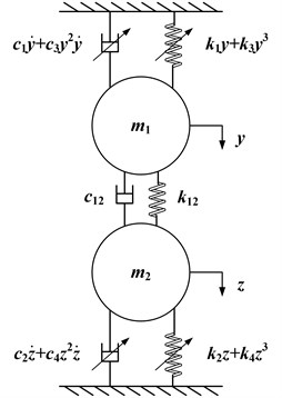
The initial vibration displacement is taken as 1 mm, 0. The initial vibration velocity is taken as , . The nonlinear stiffness coefficients , and the nonlinear damping coefficients , are taken different values. Then, the theoretical solution and CA analytical solution (CAAS) of Eqs. (1) and (2) are calculated by using MATLAB, the results are displayed in Fig. 2.
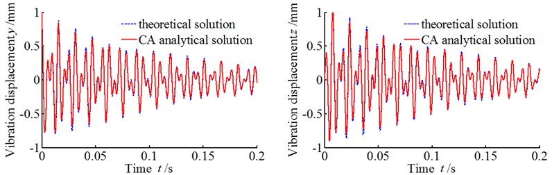
It can be seen from Fig. 2, for the linear vibration system shown in Fig. 2(a) and the weak NVS displayed in Fig. 2(b), the CAAS well coincides with the theoretical solution. And, for the strong NVS represented in Fig. 2(c), the CAAS also shows good agreement with the theoretical solution. However, as for the strong NVS revealed in Fig. 2(d), because of the nonlinear elastic force , , and the nonlinear damping force , containing high-order terms, so the nonlinear factors will have a dominant effect on vibration response. Hence, for the strong NVS which troubled by dominant nonlinear factors, there is a large error exist.
3.4. Error analysis of CA method
In order to evaluate the calculation accuracy of the CA method, it is necessary to search proper evaluation indices. Based on the previous study [30], this paper takes the average peak error, the average maximum relative error and the error of square sum as evaluation indices.
The average peak error presents the correlation degree of waveform maximum range between the CAAS and the theoretical solution, which is expressed as follows:
The average maximum relative error presents the local maximum error of calculation results, which is represented as follows:
Fig. 2Comparison between theoretical solution and CA analytical solution
a)0, 0, 0, 0
b)0.01, 0.01, 0.01, 0.01
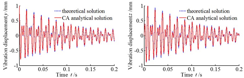
c)0.1, 0.1, 0.1, 0.1
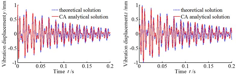
d), , ,
The error of square sum can describe the energy error between the CAAS and the theoretical solution, which is depicted as follows:
In Eqs. (31)-(33), denotes the sampling value of CAAS, is the sampling value of theoretical solution, and is the number of the sampling points.
The accuracy of the CAAS displayed in Fig. 2 is evaluated by using the above indices, and the results are depicted in table 1. Seen from table 1, as for the linear vibration system displayed in Fig. 2(a) and the weak NVS shown in Fig. 2(b), the CAAS have a high accuracy. Moreover, for the strong NVS described in Fig. 2(c), the results still have high precision. But for the strong NVS represented in Fig. 2(d), which troubled by dominant nonlinear factors, a large deviation appears. Especially, the values of and are large, and they need to be amended.
Table 1Errors of CAAS
Error value | Vibration displacement | Vibration displacement | ||||
(%) | (%) | (%) | (%) | (%) | (%) | |
0, 0, 0, 0 | 1.11 | 8.39 | 9.58 | 0.91 | 8.36 | 9.60 |
0.01, 0.01, 0.01, 0.01 | 0.80 | 8.26 | 9.66 | 0.86 | 8.25 | 9.68 |
0.1, 0.1, 0.1, 0.1 | 0.22 | 8.44 | 10.30 | 1.14 | 8.62 | 10.33 |
, , , | 0.79 | 35.34 | 12.22 | 4.97 | 37.02 | 12.43 |
4. Improvement of CA method
4.1. Basic principle of FEMD method
EMD can decompose non-stationary signals into a set of steady data series named intrinsic mode function (IMF). And IMF components must satisfy the following conditions [18]:
(1) Among the entire data set, the number of extrema and the number of zero-crossings must be equal or the difference is no more than one.
(2) At any moment, the mean value of the upper envelope formed by the local maxima and the lower envelope formed by the local minima is zero.
The purpose of the first condition is to remove the superimposed wave. The second condition changes the traditional global limit into the localized limit so that the waveform can be more symmetrical. Virtually, EMD is a screening process. Its detailed steps are as follows:
(1) All of the extreme points of the original signal are confirmed. Then, the upper and lower envelopes are calculated according to the extreme points. These two envelopes should envelop all data points.
(2) The mean of the two envelopes is denoted as . Ideally, the first IMF component of is achieved as follows:
(3) If does not meet the IMF conditions, it will be viewed as new . And the above steps (1)-(2) are repeated until corresponds with the IMF conditions.
(4) is separated from , and the remaining portion is a differential signal obtained by removing the high-frequency component from . The expression is as follows:
(5) The will be treated as a new input signal . The above steps (1)-(4) are repeated, and the second IMF component can be obtained.
(6) When the above steps (1)-(5) are repeated, then the functions from to can be gained. This process cannot be stopped until fulfils a given termination condition when is a monotonic function. Then, the decomposition formula of can be described as follows:
among them, ,…, are IMF components; is the residual component.
The above steps indicate that original signal can be decomposed by EMD to finite IMF components and a residual component. Each IMF component has different frequency-band features, and the residual component is an average trend of original signal. Meanwhile, the IMFs depend on the signal itself. Thus, EMD is a self-adaptive method.
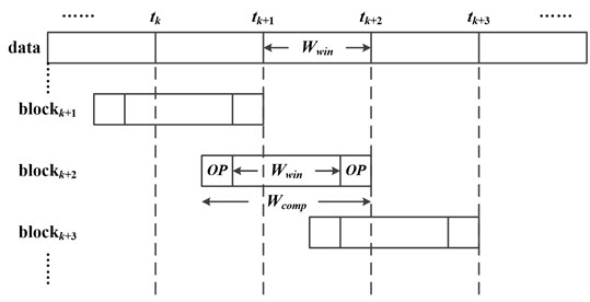
The basic idea of FEMD method is [25]: the number of decomposition mode is beforehand defined; moreover, the data series is divided by partition windows ; then, each sub-series thus generated would be sequentially processed by EMD from left to right, as demonstrated in Fig. 3. To ensure the continuity of the decomposed IMFs, the computation window is thus defined by extending on both sides with an overlap percentage (01), as described in Eq. (37). FEMD can preset the number of decomposition mode so that it can improve the calculation speed and effectively suppress the mode mixing phenomenon:
Fig. 3The diagram of FEMD method
4.2. Relation between FEMD and CA
Firstly, the theoretical solutions exhibited in Fig. 2(a) are calculated by fast Fourier transform (FFT), the results are shown in Fig. 4. The results indicate that the natural frequencies of system are 126 Hz, 192 Hz, and the corresponding natural angular frequencies are 791.6813 rad/s, 1206.3716 rad/s.
Secondly, the theoretical solutions revealed in Fig. 2(a) are decomposed by FEMD method, and some IMF components are acquired. Then, the phase information of each IMF is obtained by using Hilbert transform method. Furthermore, the instantaneous frequency of each IMF is achieved according to Eq. (38), and the results are displayed in Fig. 5.
After calculation, the mean instantaneous frequencies of IMF1, IMF2 decomposed from y are 191.5904 Hz and 125.5786 Hz. The mean instantaneous frequencies of IMF1, IMF2 decomposed from are 191.9599 Hz and 125.6273 Hz. Compared with the natural frequencies obtained by FFT, the mean instantaneous frequency of IMF1 corresponds to the natural frequency , and the mean instantaneous frequency of IMF2 is corresponding to the natural frequency . So, IMF1 and IMF2 are the inherent mode components of system.
Fig. 4Amplitude spectrum of vibration displacement signal
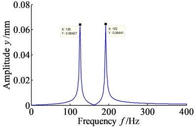
a) Vibration displacement
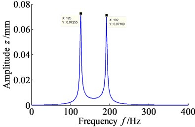
b) Vibration displacement
Fig. 5Time-frequency spectrum of vibration displacement signal
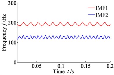
a) Vibration displacement

b) Vibration displacement
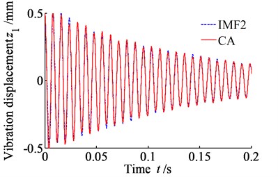
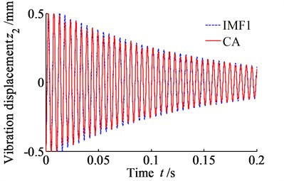
In order to further explore the connection between FEMD and CA, the IMF components acquired by FEMD are compared with the analytical solutions obtained by CA. The results are represented in Fig. 6 and Fig. 7.
Fig. 6Comparison between IMF component and CAAS derived from y
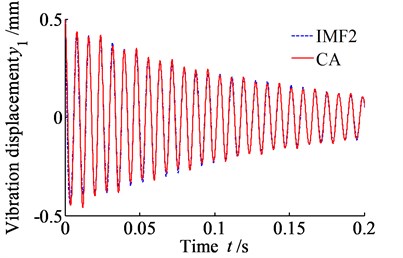
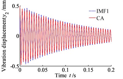
It can be seen from Fig. 6 and Fig. 7, the CAAS are consistent with the IMF component. So, the amplitude and phase of them should have one-to-one relationship. Hence, when deviation appears in CA method influenced by nonlinear factors, the amplitude and phase of CAAS can be modified by FEMD method.
Fig. 7Comparison between IMF component and CAAS derived from z
The theoretical connection between FEMD method and CA method is further derived. If the IMF components obtained by FEMD are processed by Hilbert transform, there are:
Then, the analytic signal of IMF component can be constructed by and . Its expression is as follows:
where amplitude , phase .
According to the above analysis, the relationship between the IMF component and the CAAS can be acquired from Eq. (40), Eq. (29) and Eq. (30). Its expression can be depicted by:
Moreover, according to Eq. (41) and mathematical transformation , the modified expressions of the slow-varying amplitude and slow-varying phase angle derived from CAAS can be further obtained. Their expressions can be given by:
4.3. Correction for CA analytical solution
Based on the above analysis and theoretical derivation, the detailed steps of the correction for CAAS can be described as follows:
(1) The vibration response of the system is tested to obtain a set of vibration displacement signals.
(2) The vibration displacement signals are individually processed by FFT to acquire the natural frequency and natural angular frequency .
(3) The vibration displacement signals are also individually decomposed by FEMD to achieve a number of IMF components.
(4) The instantaneous frequency of each IMF component is computed and further compared with the natural frequency acquired by FFT. Then, the IMF components which can represent the natural frequency of system are selected.
(5) The selected IMF components are processed by Hilbert transform to obtain the slow-varying amplitude and slow-varying phase .
Fig. 8Comparison between theoretical solution and CA corrected solution
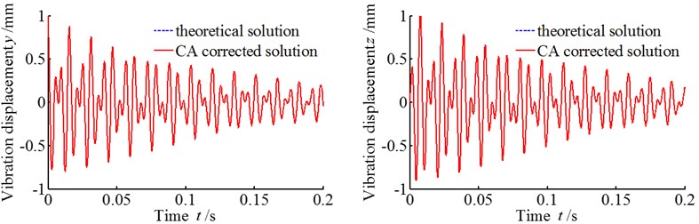
a)0, 0, 0, 0
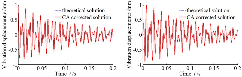
b)0.01, 0.01, 0.01, 0.01
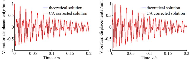
c)0.1, 0.1, 0.1, 0.1
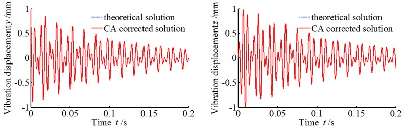
d), , ,
(6) The parameters of the slow-varying amplitude and slow-varying phase angle are corrected by utilizing the modified expressions Eqs. (42) and (43). Afterwards, the corrected , and the natural angular frequency are substituted into the Eqs. (29) and (30). Then, an accurate CAAS can be acquired.
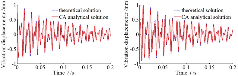
By using the above method, the CAAS described in Fig. 2 are modified, and the corrected results are shown in Fig. 8.
Similarly, the accuracy of the CA corrected solutions depicted in Fig. 8 is evaluated by using the error indices, and the results are displayed in Table 2.
Table 2Errors of CA corrected solution
Error value | Vibration displacement | Vibration displacement | ||||
(%) | (%) | (%) | (%) | (%) | (%) | |
0, 0, 0, 0 | 1.81×10⁻¹⁶ | 3.07×10⁻¹⁴ | 3.61×10⁻¹⁶ | 3.34×10⁻¹⁶ | 3.20×10⁻¹⁴ | 2.91×10⁻¹⁶ |
0.01, 0.01, 0.01, 0.01 | 0 | 3.12×10⁻¹⁴ | 1.98×10⁻¹⁵ | 6.14×10⁻¹⁷ | 3.25×10⁻¹⁴ | 2.18×10⁻¹⁵ |
0.1, 0.1, 0.1, 0.1 | 1.11×10⁻¹⁶ | 3.14×10⁻¹⁴ | 1.81×10⁻¹⁶ | 2.50×10⁻¹⁶ | 3.23×10⁻¹⁴ | 2.91×10⁻¹⁵ |
, , , | 1.89×10⁻¹⁶ | 3.27×10⁻¹⁴ | 1.68×10⁻¹⁵ | 1.64×10⁻¹⁶ | 3.43×10⁻¹⁴ | 1.51×10⁻¹⁶ |
Comparing Table 2 and Table 1, whether for weak NVS or strong NVS, the CA corrected solutions have high precision. The errors between the theoretical solutions and CA corrected solutions are small. Especially, as for the strong NVS (, , , ) which is troubled by dominant nonlinear factors, the errors are significantly reduced. The results indicate that the CAAS can be effectively corrected by utilizing FEMD method, and the accuracy of the solution can be significantly improved.
5. Conclusions
On the basis of theoretical research, the nonlinear vertical vibration model of MRS is established. And the analytical solution of the model is explored. Through theoretical research and numerical experiment analysis, the following conclusions are obtained:
(1) The CA method has a high accuracy in solving linear vibration system and weak NVS. As for strong NVS, because of the nonlinear elastic force and the nonlinear damping force containing high-order terms, the nonlinear factors have a dominant effect on system vibration response. So, the CAAS will have a large error while system is troubled by dominant nonlinear factors, which needs to be modified.
(2) The FEMD can decompose non-stationary signals into some IMF components. The amplitude and phase between CAAS and the selected IMF component have specific relationship. Hence, when deviation appears in CA method influenced by nonlinear factors, the amplitude and phase of CAAS can be modified by FEMD method. Results indicate that CAAS can be effectively corrected by utilizing FEMD method, and the accuracy can be significantly improved. The improved CA method can be used to solve strong NVS with two DOF.
References
-
Hameed W. I., Mohamad K. A. Strip thickness of cold rolling mill with roll eccentricity compensation using fuzzy neural network. Engineering, Vol. 6, 2014, p. 27-33.
-
Tran D. C., Tardif N., Limam A. Experimental and numerical modeling of flatness defects in strip cold rolling. International Journal of Solids and Structures, Vol. 69-70, 2015, p. 343-349.
-
Zhang Y. J., Shen G. X., Li Y. G., et al. Spatial vibration and its numerical analytical method of four-high rolling mills. International Journal of Iron and Steel Research, Vol. 21, Issue 9, 2014, p. 837-843.
-
Zárate L. E., Bittencout F. R. Representation and control of the cold rolling process through artificial neural networks via sensitivity factors. Journal of Materials Processing Technology, Vol. 197, Issues 1-3, 2008, p. 344-362.
-
Yang X., Tong C. N., Yue G. F., et al. Coupling dynamic model of chatter for cold rolling. International Journal of Iron and Steel Research, Vol. 17, Issue 12, 2010, p. 30-34.
-
Schausberger F., Steinboeck A., Kugi A. Mathematical modeling of the contour evolution of heavy plates in hot rolling. Applied Mathematical Modelling, Vol. 39, Issue 15, 2015, p. 4534-4547.
-
Zhu Y., Jiang W. L., Kong X. D., et al. Study on nonlinear dynamics characteristics of electro-hydraulic servo system. Nonlinear Dynamics, Vol. 80, Issues 1-2, 2015, p. 723-737.
-
Novak N., Vladimir S., Vladimir D. Optimal control of hydraulically driven parallel robot platform based on firefly algorithm. Nonlinear Dynamics, Vol. 82, Issue 3, 2015, p. 1457-1473.
-
Navarro J. F. On the implementation of the Poincaré-Lindstedt technique. Applied Mathematics and Computation, Vol. 195, Issue 1, 2008, p. 183-189.
-
Lakrad F., Belhaq M. Periodic solutions of strongly non-linear oscillators by the multiple scales method. Journal of Sound and Vibration, Vol. 258, Issue 4, 2002, p. 677-700.
-
Zhang C. L., Harne R. L., Li B., et al. Reconstructing the transient, dissipative dynamics of a bistable Duffing oscillator with an enhanced averaging method and Jacobian elliptic functions. International Journal of Non-Linear Mechanics, Vol. 79, 2016, p. 26-37.
-
Cai J. P., Wu X. F., Li Y. P. Comparison of multiple scales and KBM methods for strongly nonlinear oscillators with slowly varying parameters. Mechanics Research Communications, Vol. 31, Issue 5, 2004, p. 519-524.
-
Farzaneh Y., Tootoonchi A. A. Global error minimization method for solving strongly nonlinear oscillator differential equations. Computers and Mathematics with Applications, Vol. 59, 2010, p. 2887-2895.
-
Hosen M. A., Chowdhury M. S. H. A new reliable analytical solution for strongly nonlinear oscillator with cubic and harmonic restoring force. Results in Physics, Vol. 5, 2015, p. 111-114.
-
Razzak M. A., Molla M. H. U. A new analytical technique for strongly nonlinear damped forced systems. Ain Shams Engineering Journal, Vol. 6, Issue 4, 2015, p. 1225-1232.
-
Manevitch L. I. Complex representation of dynamics of coupled nonlinear oscillators. Mathematical Models of Nonlinear Excitations, Transfer Dynamics and Control in Condensed Systems, 1999, p. 269-300.
-
Kerschen G., Vakakis A. F., Lee Y. S., et al. Toward a fundamental understanding of the Hilbert-Huang transform in nonlinear structural dynamics. Journal of Vibration and Control, Vol. 14, Issues 1-2, 2008, p. 77-105.
-
Huang N. E., Shen Z., Long S. R., et al. The empirical mode decomposition and the Hilbert spectrum for nonlinear and nonstationary time series analysis. Proceedings of Royal Society of London A, Vol. 454, 1998, p. 903-995.
-
Shaw P. K., Saha D., Ghosh S., et al. Investigation of coherent modes in the chaotic time series using empirical mode decomposition and discrete wavelet transform analysis. Chaos, Solitons and Fractals, Vol. 78, 2015, p. 285-296.
-
Gupta P., Sharma K. K., Joshi S. D. Fetal heart rate extraction from abdominal electrocardiograms through multivariate empirical mode decomposition. Computers in Biology and Medicine, Vol. 68, 2016, p. 121-136.
-
Lei Y. G., Lin J., He Z. J., et al. A review on empirical mode decomposition in fault diagnosis of rotating machinery. Mechanical Systems and Signal Processing, Vol. 35, Issues 1-2, 2013, p. 108-126.
-
Xie X. H. Illumination preprocessing for face images based on empirical mode decomposition. Signal Processing, Vol. 103, 2014, p. 250-257.
-
Fan G. F., Peng L. L., Hong W. C., et al. Electric load forecasting by the SVR model with differential empirical mode decomposition and auto regression. Neurocomputing, Vol. 173, 2016, p. 958-970.
-
Wu Z., Huang N. E. Ensemble empirical mode decomposition: a noise-assisted data analysis method. Advances in Adaptive Data Analysis, Vol. 1, Issue 1, 2009, p. 1-41.
-
Wang Y. H., Yeh C. H., Young H. V., et al. On the computational complexity of the empirical mode decomposition algorithm. Physica A, Vol. 400, Issue 15, 2014, p. 159-167.
-
Hou D. H., Chen H., Liu B., et al. Analyze on nonlinear parametrically exited vibrations of roller system. Journal of Vibration and Shock, Vol. 28, Issue 11, 2009, p. 1-5.
-
Meng L. Q., Du Y., Ma S. B., et al. Non-linearity of vertical vibration of medium plate mill. Journal of Jilin University, Vol. 39, Issue 3, 2009, p. 712-715.
-
Chen Y. H., Shi T. L., Yang S. Z. Study on parametrically excited nonlinear vibrations on 4-H cold rolling mills. Journal of Mechanical Engineering, Vol. 39, Issue 4, 2003, p. 56-60.
-
Liu H. R., Shi P. M., Chen H., et al. Study on nonlinear parametrically exited coupling vibrations of roller system on 4-H rolling mills. China Mechanical Engineering, Vol. 22, Issue 12, 2011, p. 1397-1401.
-
Zhu Y., Jiang W. L., Kong X. D., et al. An accurate integral method for vibration signal based on feature information extraction. Shock and Vibration, Vol. 2015, 2015, p. 1-13.
Cited by
About this article

This work is supported by National Natural Science Foundation of China (No. 51475405), National Key Basic Research Program (973 Program) of China (No. 2014CB046405), Innovation Foundation for Graduate Students of Hebei Province (00302-6370002) and Natural Science Foundation of Hebei Province (E2017203039).
