Abstract
A method based on multiscale base-scale entropy (MBSE) and random forests (RF) for roller bearings faults diagnosis is presented in this study. Firstly, the roller bearings vibration signals were decomposed into base-scale entropy (BSE), sample entropy (SE) and permutation entropy (PE) values by using MBSE, multiscale sample entropy (MSE) and multiscale permutation entropy (MPE) under different scales. Then the computation time of the MBSE/MSE/MPE methods were compared. Secondly, the entropy values of BSE, SE, and PE under different scales were regarded as the input of RF and SVM optimized by particle swarm ion (PSO) and genetic algorithm (GA) algorithms for fulfilling the fault identification, and the classification accuracy was utilized to verify the effect of the MBSE/MSE/MPE methods by using RF/PSO/GA-SVM models. Finally, the experiment result shows that the computational efficiency and classification accuracy of MBSE method are superior to MSE and MPE with RF and SVM.
1. Introduction
In the mechanical system, a basic but important component is roller bearings, whose working performance has great effects on operational efficiency and safety. Two key parts of the roller bearing fault diagnosis, are characteristic information extraction and fault identification.
For the information extraction, the roller bearings vibration signals are essential. It should be noted that the fault diagnosis is challenging in the mechanical society as the vibration signals are unstable.
Owing to the roller bearings vibration signals are nonlinear, many nonlinear signal analysis methods including fractal dimension, approximate entropy (AE) and sample entropy (SE) have been proposed, and applied in different domains, such as physiological, mechanical equipment vibration signal processing, and chaotic sequence [1-4]. Pincus et. al presented a model named AE to analysis time series signals [5, 6], but the AE model exists some problems, such as the AE model is sensitive to the length of the data. Therefore, the value of AE is smaller than the expected value when the length of the data is very short. To overcome this disadvantage, an improved method based on AE, called SE, was proposed in [7], AE has been successfully used in fault diagnosis [8]. It is different from AE and SE, Bandt et al. presented PE, a parameter of average entropy, to describe the complexity of a time series [9]. Because the permutation entropy makes use of the order of the values and it is robust under a non-linear distortion of the signal. Additionally, it is also computationally efficient. The PE method has been successfully applied in rotary machines fault diagnosis [10]. Compared with SE, the computational efficiency of PE is superior to the SE, because SE requires to calculate the entropy value using increase the dimension to for sequence reconstruction, but PE takes only once for sequence reconstruction. However, before PE entropy value calculation, the time sequence should be sorted, the computational efficiency of the SE and PE methods are both not good. Therefore, a method, named base-scale entropy (BSE) was presented. In [11], the authors demonstrated that the computational efficiency of the BSE is good, and applied in physiological signal processing and gear fault diagnosis successfully [12, 13].
It should be noted that SE and PE can only reflect the irregularity of time series on a single scale. A method called multiscale entropy (ME) is proposed to measure time sequence irregularity [14, 15], in which the degree of self-similarity and irregularity of time series can be reflected in different scales. For example, the outer race fault and the inner race fault vibration signals can be identified respectively according to the characteristics of the spectrum when roller bearings running at a particular frequency. The frequencies of vibration signals have deviations when the roller bearings failure occurs, and the corresponding complexity also has differences. Therefore, ME can be regarded as a characteristic index for fault diagnosis [16]. Based on the multiscale sample entropy (MSE), the feature of the vibration signals can be extracted under various conditions, then the eigenvector is regarded as the input of adaptive neuro-fuzzy inference system (ANFIS) for roller bearings fault recognition [17]. In [18], a method called multiscale permutation entropy (MPE) is applied in feature extraction, and then extracted features are given input to the adaptive neuro fuzzy classifier (ANFC) for an automated fault diagnosis procedure.
As the rapid development of computer engineering techniques, many fault recognition methods including support vector machine (SVM) [19, 20] and random forests (RF) [21] models, are utilized in fault diagnosis. Furthermore, an existed difficulty is the selection proper SVM parameters in order to obtain the optimal performance of SVM. These parameters that should be optimized include the penalty parameter C and the kernel function parameter g for the radial basis kernel function (RBF). The SVM with particle swarm optimization (PSO) [22-25] and Genetic Algorithm (GA) [26]. However, RF is one of recently emerged ensemble learning methods, since firstly introduced by Leo Breiman [21]. The RF method runs efficiently on large datasets, and it estimates missing data accurately and even retains accuracy when a large portion of the data is missing. Hence, the RF model is chosen as the classifier in this study.
As mentioned above, combining multiscale base-scale entropy (MBSE) and RF, a method based on MBSE and RF was presented in this paper. Firstly, the MBSE/MSE/MPE methods were used to compute the BSE, SE, and PE entropy values for roller bearing’s vibration signals, and then the comparison of the computation time of the MBSE/MSE/MPE methods were analyzed. Secondly, the values of BSE, SE, and PE under different scales were regarded as the input of RF/SVM models for fulfilling the fault identification, and the classification accuracy was used to verify the effect of the MBSE/MSE/MPE methods with RF/SVM models. Finally, the experiment result shows that the classification accuracy and computational efficiency of MBSE-RF are better than MPE/MSE-RF/SVM and MBSE-SVM models.
The rest of this paper is organized as follows: The theoretical framework of MBSE and RF are shown in Section 2, The experimental data sources, procedures of the proposed method and parameter selection for different methods are described in Section 3. Experimental results and analysis are given in Section 4 followed by conclusions in Section 5.
2. Theoretical framework of MBSE and RF
2.1. Basic principle of MBSE
The basic principle of MBSE comes from BSE using the reconstruction and multi-scale calculation operations. The detailed theoretical framework of BSE is given in [11, 12].
(1) BSE: The procedures of BSE calculation are given as follows:
Step 1: For a given time series with points . Firstly, the time series should be constructed in the following formula:
where contain consecutive values, thence there are vectors with -dimension in .
Step 2. The root mean square of each two adjacent samples and with -dimensional are used to calculate the BS value:
Step 3: Transforming each -dimensional vector into the symbol vector set , . The standard of the symbol vector set is according to the following formula:
where represent mean value of the th vector here a is a constant value. The symbol set sequences are employed to calculate the distributed probability for each vector .
Step 4: Owing to the different composite states in vector and the number of symbol is 4. So, the number of composite states is . It should be noted that each state denotes a mode. The detailed calculation of as follows:
where .
Step 5: The BSE value is calculated by:
(2) MBSE: The basic principle of MBSE comes from BSE using the multiscale operation, because the BSE compute the entropy only for single scale. ME uses the multiscale values to reflect the irregularity and self-similarity trend of the data, MBSE is combine the ME and BSE. Therefore, the calculation process of MBSE as follows:
For the aforementioned time series . The procedures of the coarse-grained operation is calculated by:
where denotes the scale factor. It should be noted that the coarse-grained time series is the original time series when 1. Hence a coarse-grained vector series are the results of the original time series through coarse-grained operation. After the coarse-grained operation, the length and number of the are and , respectively.
As mentioned above, those operations including Step 1 to Step 7 is MBSE calculation.
2.2. Basic principle of decision tree and RF models
2.2.1. Decision tree (DT)
DT is one of the commonly tools for classification and prediction tasks, it is based on attribute space, by using the iterative procedure of binary partition providing a highly interpretable method.
For a given data set with samples, here , for each sample has input attributes, such as , is the classification label of the . The is an identifier indicate the corresponding class , therefore, means that the sample belongs to the class . The procedure of selecting attributes and partition was described in detail in reference [27].
For the overall data, an attribute and the partition points are selected, hence the pair of semiplanes and is defined as follows:
We regard the parameter as the proportion of observations of class in the region , regarding the overall observations into this region:
where , here is membership indicator of the attribute vector to that region. is a homogeneity measure of the child nodes, also called the impurity function. Other impurity functions are defined by them is classification error, the Gini index and the cross-entropy or deviance. The iterative procedure splits the attribute space into disjoints regions , as far as the stop criterion is reached. The class is assigned to node of the tree, which represents the region , that is, . This procedure searches throughout all possible values of all attributes among the samples.
The binary tree method is used in DT, the mother mode in DT represents the original partition on the domain of the selected attribute, then the corresponding child nodes represents the original partition on the domain of the selected attribute. The leaf nodes represent the sample classification. In order to obtain the semiplanes and in DT, the partition rules for selecting the is described in reference [27].
Aiming at solving the problem of high variance, therefore, the bagging tool is used to solve this problem. The bagged classifier is composed of a set of decision trees which are built from the random subsets of available data samples, hence the predicted class is proposed from this set of classifiers. Here and represents the class and the classifier proposing the class for the input sample , the overall sample classification depends on the largest number of “votes” that are proposed for each classifier , it is defined as:
where is the predicted class, is the vector , in which represents the partition of the estimators proposing the class .
2.2.2. Random forest (DT)
Random forests (RF) is one of recently emerged ensemble learning methods. A random forest is a classifier consisting of a collection of tree-structured classifiers , . The RF classifies anew object from an input vector by examining the input vector on each decision tree (DT) in the forest.
The process to decrease the variance, by reducing the correlation between the trees, is accomplished through the random selection of the input variables and the random selection with replacement of samples from the data set of size . The selected variables and samples are used to grow every tree in the forest (bootstrap sample). This random selection has shown that around 2/3 of the data are chosen, then, the training set for each classifier is, in general, . The RF algorithm for the classification problem is summarized in reference [21].
The entire algorithm includes two important phases: the growth period of each DT and the voting period.
(1) Growth of trees: If the number of cases in the training set is , sample cases as random-but with replacement from the original data. This sample will be the training set for growing the DT. At each node, variables are randomly selected out of the input variables () and the best split on these is used to split the node. The value of is held constant during the forest growing. Each DT is grown to the largest extent possible. No pruning is applied.
(2) Voting: In random forest algorithm, the predication of new test data is done by majority vote. New test data runs down all trees in the ensemble, and the classification of each data point is recorded for each tree, then using majority vote, the final classification given to each data point is the class that receives the most votes across all trees. A user-defined threshold can loosen this condition. As long as the number of the votes for a certain class A is above the threshold, it can be classified as class A. Once the RF is obtained, the decision for classifying a new sample is according to the following equation:
where is the class that is assigned by the tree .
3. Experimental data sources, procedures of the proposed method and parameter selection
3.1. Experimental data sources
In this section, we introduce the experimental data, the roller bearings fault datasets come from the Case Western Reserve University [8]. The detailed description of the dataset is given in [17], the datasets were collected by accelerometer which was fixed on Drive End (DE) and Fan End (FE) of a motor. The sampling frequency is 12000 Hz. The collected signals are divided into four types of faults with various diameters: normal (NR), ball fault (BF), inner race fault (IRF), and outer race fault (ORF). The fault diameter contains 0.1778 mm, 0.3556 mm, and 0.5334 mm. In order to distinguish the degree of fault, we divided the fault into four categories: normal, slight, moderate, and server. The length of each sample is 2048, the total number of the sample is 600, 12 different types of failures were used in this paper. The detailed description of the experimental data is given in Table 1.
Table 1The roller bearings experimental data under different conditions
Fault category | Fault diameters (mm) | Motor speed (rpm) | Number of samples | The fault severity |
NR1 | 0 | 1750 | 50 | Normal |
IRF1 | 0.1778 | 1750 | 50 | Slight |
BF1 | 0.1778 | 1750 | 50 | Slight |
ORF1 | 0.1778 | 1750 | 50 | Slight |
NR2 | 0 | 1730 | 50 | Normal |
IRF2 | 0.3556 | 1730 | 50 | Moderate |
BF2 | 0.3556 | 1730 | 50 | Moderate |
ORF2 | 0.3556 | 1730 | 50 | Moderate |
NR3 | 0 | 1797 | 50 | Normal |
IRF3 | 0.5334 | 1797 | 50 | Server |
BF3 | 0.5334 | 1797 | 50 | Server |
ORF3 | 0.5334 | 1797 | 50 | Server |
3.2. Procedures of the proposed method
In this Section, the procedures of the proposed method can be described as follows.
Step 1: Preprocessing vibration signals under different scales factor by using MBSE/MSE/MPE models. The different parameters of SE/PE/BSE according to the Section 3.3 to compute the different entropy values.
Step 2: Selecting the different parameters in PSO/GA-SVM and RF models according to the Section 3.3.
Step 3: Calculating the MBSE, MPE, and MSE entropy values. All these values are regarded as samples which are divided into two subsets, the training and testing samples. Meanwhile, comparing the elapsed time by using MBSE, MSE and MPE respectively.
Step 4: The eigenvectors MSE1-MSE20/MPE1-MP220/MBSE1-MBSE20 are regarded as input of the trained PSO/GA-SVM and RF models and then the different vibration signals can be identified by the output of the RF/SVM classifiers.
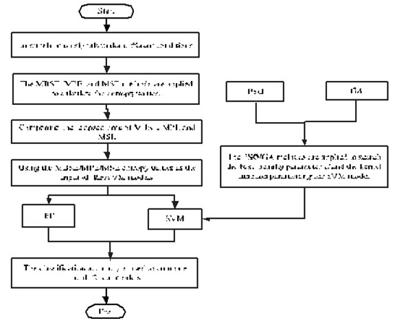
Step 5: The classification accuracy is used to compare the different models. The flowchart to of parameter selection for different methods are given in Fig. 1
Fig. 1The flowchart to of parameter selection for different methods
3.3. Parameter selection for different methods
(1) BSE: The authors suggested set the embedded dimension in Eq. (4) as 3 to 7. Because the length of the data meeting the condition , the larger the value, the harder the meeting the condition. Set the m value exceed 7 will result in losing some important information of the original data. The parameter in Eq. (3) is often fixed as 0.1-0.4. Additionally, the larger the value , the more detailed reconstruction of the dynamic process. We set as 4 and 5 and fixed as 0.2 and 0.3 in this paper [11].
(2) Some parameters including embedded dimension and the time delay should be preset before PE calculation. The time delay parameter has little effect on PE calculation, it is often set as 1. The most of the important parameter is dimension . In general, the more the value , the easier to homogenize vibration signals, the smaller the value , the more difficult to detect the vibration signals exactly [9]. Therefore, the embedded dimension is selected as 3, 4, 5, and 6. The time delay parameter 1 in this paper.
(3) SE: There are two parameters, such as parameter embedding dimension , similarity tolerance , need to set before the SE calculation. In general, the function of the embedding dimension is the same as the PE, but in SE, this parameter needs to meeting the condition -, here is the length of the data. Therefore, we use 2 in this paper [7, 17]. The similarity tolerance is used to determine the gradient and range of the data. Too small value will lead to salient influence from noise. Meanwhile, too a large value will result in lose some useful information from noise. Experimentally, is often set as the multiplied by the standard deviation (SD) of the original data [3, 17]. We use 0.15SD, 0.2SD, and 0.25SD in this paper.
(4) The length of each sample is selected as 2048 in this paper, the scale factor in MBSE, MPE and MSE methods is often fixed as 20 [17, 18].
(5) RF: Two parameters should be set before the RF model training, such as is selected according to the input variables. After extracting MBSE/MSE/MPE as feature vectors and the scale factor is fixed as 20, so the number of input variables 20, and the parameter is often meet the condition [21], the 4 and the number of the DT are fixed as 4 and 500 in this paper.
(6) PSO: The basic principle of the PSO and SVM was given in detail in [19]. The size of particles is chosen as 20. The maximum iteration number 200 and the termination tolerance 1-3. The velocity and position are restricted to the [0.01, 1000] and [0.1,100], positive constant and are fixed as 1.5 and 1.7, and are random numbers in the range of [0,1]. The kernel function is selected as radial basis function (RBF) in SVM model. The fitness function is used to evaluate the quality of each particle which must be designed before searching for the optimal values of the SVM parameters.
(7) GA: The basic principle of the GA was described in detail in [26]. The size of population is set as 20 and maximum iteration number 200, termination tolerance 1e-3. The crossover and the mutation probability are set as 0.7 and 0.035 respectively. The penalty parameter and kernel function parameter are regarded as optimization options in PSO/GA models.
(8) The fitness function is based on the classification accuracy of a SVM classifiers, which can be set as follows: fitness function = 1– sum error / (sum right + sum error), here sum error and sum right indicate the number of true and false classifications respectively
4. Experimental results and analysis
4.1. Simulation analysis of experimental data
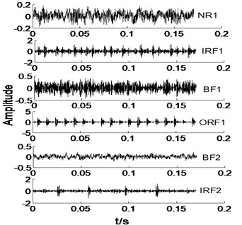
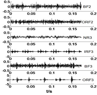
In this section, we select the all signals in Table 1 with a sample for an example, thence the time domain of original signals under different condition are given in Fig. 2.
Fig. 2The time domain waveforms of vibration signals under different working conditions
a)
b)
As shown in Fig. 2, it is difficult to distinguish the all signals, take NR1 and BF signals for an example. Owing to the NR signals without regularity, thence the NR signals are very complicated, and BF signals also is. However, IRF and ORF signals have a certain degree of regularity, but it is not easy to distinguish at a glance. Most of the various signals have same vibration amplitude, such as BF1-BF3 and ORF1-ORF3. Therefore, the MBSE, MPE, and MPE models are used to calculate the entropy values and observe its complex trends in Fig. 2 under different scales. The results of MBSE, MSE, and MPE are shown in Fig. 3.
4.2. The comparison of MSE/MPE/CMPE computational efficiency
Then computing the total and average elapsed time for MBSE, MPE and MSE methods with 600 samples, therefore, the corresponding results of MBSE ( 4, 0.3), MPE ( 4) and MSE ( 0.2SD) methods are given in Table 2.
Table 2The total and average elapsed time for MBSE, MPE and MSE methods with 600 samples
Computation time | MBSE | MPE | MSE |
The total elapsed time (s) | 56.762665 | 115.203234 | 109.218942 |
The average elapsed time (s) | 0.09460444 | 0.19200539 | 0.18203157 |
It can be seen from Table 2, the smallest total and average elapsed time are 56.762665 and 0.09460444, this indicates that the computational efficiency of MBSE is better than MPE and MSE models. The corresponding reasons are given as follows:
(1) For a given signal , the length of the is . In the reconstruction process, -dimensional vector need to be reconstructed. Compared with SE, in which requires increase the to for signal reconstruction, thence is has twice reconstruction operation. But BSE and PE need once reconstruction operation.
(2) In BS value calculation procedure, the number of addition, subtraction, multiplication, and division operations are , , , and according to the Eq. (2). Before calculation, the mean value of each is calculated, thence the number of addition and division operations are , . When computing the in the following step, the corresponding cycle number of addition, subtraction, multiplication and comparison (“>”, “<” and “=”) operations, are , , , . For each -dimensional vector , the probability is counted. The number of comparison and division operations under different state are and . Lastly, for BSE entropy calculation, the number of addition, multiplication and logarithm operations are , , .
(3) Each adjacent data points are sorted before PE calculation, thence the number of comparison operation is . For each -dimensional vector . The composite states should be counted in vector [9, 10]. To find the states . In each -dimensional vector , the comparison and division operations are needed to count, owing to the kinds of states are included in all vectors , thence the number of operations is and (N-m+1). Lastly, in order to calculate the PE entropy value, several types of operation, such as addition, multiplication and logarithm, are used to compute the PE value. The corresponding operation number are , , .
(4) The detailed calculation process of SE is given in [7, 8, 17]. Using the distance to calculate any two sample points and . Hence the number of subtraction operation is . In order to count up the number of , in which is meet the conditions [7]. In this step, comparison operation (< and =) with cycles are needed. Several kinds of operations, such as addition, multiplication and division, are used to calculate the [7]. Additionally, the same operations in , are considered to compute the by increase the to .
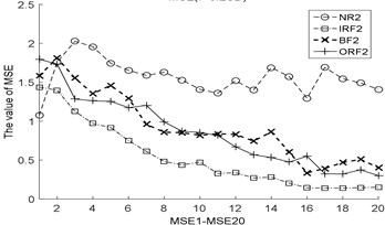
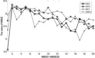
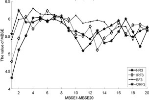
Fig. 3The MBSE/MSE/MPE values (MBSE1-MBSE20/MSE1-MSE20/MPE1-MPE20) under different conditions
a) MSE, 0.2SD

b) MSE, 0.2SD

c) MSE, 0.2SD
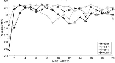
d) MPE, 4
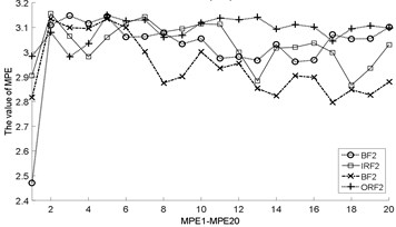
e) MPE, 4
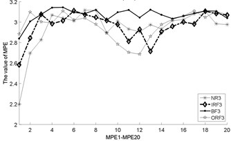
f) MPE, 4
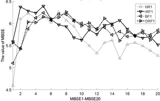
g) MBSE, 4, 0.3
h) MBSE, 4, 0.3
i) MBSE, 4, 0.3
The total cycle number of BSE, PE, and SE using different operations are given in Table 3.
As shown in Table 3, the total cycle number of BSE is , which is smaller than the PE/SE methods. Therefore, the computational efficiency of BSE is faster than PE/SE methods. In order to calculate the ME values combining BSE, PE, and SE, this operation will lead to increase the computation time gap in MBSE/MPE/MSE methods when calculating BSE, PE and SE values under each scale, the computational efficiency of MBSE method is superior than MPE and MSE methods.
Table 3The total number of addition, subtraction, multiplication, division, and comparison operations of BSE/PE/SE models
Operation | BSE | PE | SE |
+ | 2( 1) | ( 1) | 2( 1) |
– | ( 1) | – | 2()( 1) |
* | ( 1)( 1) | ( 1) | 2( 1) |
/ | 3( 1) | ( 1) | 2( 1) + 3 |
log | ( 1) | ( 1) | 1 |
>, <, = | 2()( 1) | ||
Total |
4.3. Fault identification
After extracting MBSE/MSE/MPE as feature vectors, this data is divided in to training and testing samples for automated roller bearings fault diagnosis. For each working condition (50 samples) in Table 1. In this paper, 20, 30, 40 samples were selected as training samples for MBSE/MSE/MPE-RF/SVM models respective. The corresponding total number of training samples is 240, 360 and 480, and the rest 40, 30, 20 samples are selected as testing data for verify the accuracy of MBSE/MSE/MPE-RF models respectively. The corresponding number of training samples is 480, 360 and 240. Fig. 4 shows the desired output and the output of the trained MBSE/MSE/MPE-RF/SVM models. The results of classification accuracy and average accuracy of the MBSE/MSE/MPE-RF/SVM models are given in Table 4 and Table 5. (As limited space, here some fault classification figures are given in Fig. 5).
Table 4The results of the classification accuracy by using MBSE/MSE/MPE-RF/SVM models
Mode | Accuracy (%) | Average accuracy (%) | Total average accuracy (%) | ||
Total testing samples No. | |||||
240 | 360 | 480 | |||
MBSE-RF ( 4, 0.2) | 99.58 | 99.16 | 98.75 | 99.16 | 97.17 |
MBSE-RF ( 4, 0.3) | 97.08 | 96.66 | 96.45 | 96.73 | |
MBSE-RF ( 5, 0.2) | 97.5 | 96.11 | 95.62 | 96.41 | |
MBSE-RF ( 5, 0.3) | 97.08 | 96.11 | 96.04 | 96.41 | |
MPE-RF ( 3) | 96.25 | 96.66 | 94.58 | 95.83 | 96.88 |
MPE-RF ( 4) | 97.91 | 98.33 | 97.91 | 98.05 | |
MPE-RF ( 5) | 97.08 | 97.22 | 97.08 | 97.12 | |
MPE-RF ( 6) | 96.66 | 95.83 | 97.08 | 96.52 | |
MSE-RF ( 0.15SD) | 92.5 | 86.66 | 85.62 | 88.26 | 90.78 |
MSE-RF ( 0.2SD) | 91.38 | 88.05 | 85 | 88.14 | |
MSE-RF ( 0.25SD) | 96.66 | 94.58 | 96.66 | 95.96 | |
(1) It can be seen from Table 4 and Table 5 that the highest classification accuracy is up to 99.58 % when 4, 0.2 by using MBSE-RF models.
(2) As shown in Table 4 and Table 5, the classification accuracy and average accuracy of RF model is higher than PSO/GA-SVM under different conditions. For example, 99.16 % is the highest average accuracy in Table 4 when 4 and 0.2 by using MBSE-RF model.
Fig. 4The results of fault classification between the actual and predict samples by using MBSE/MPE/MSE-RF/SVM models
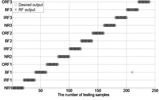
a) MBSE-RF ( 4, 0.2)
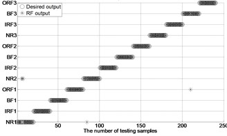
b) MPE-RF ( 4)
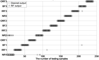
c) MSE-RF ( 0.2SD)

d) MBSE-PSO-SVM ( 4, 0.2)
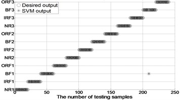
e) MPE-PSO-SVM ( 4)
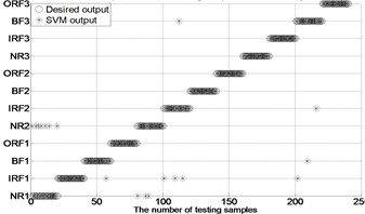
f) MSE-PSO-SVM ( 0.2SD)
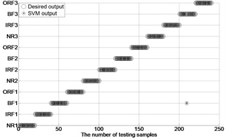
g) MBSE-GA-SVM ( 4, 0.2)
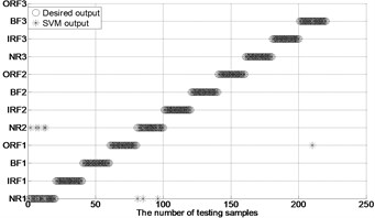
h) MPE-GA-SVM ( 4)

i) MSE-GA-SVM ( 0.2SD)
(3) The classification accuracy and average accuracy of MBSE model is higher than MPE/MSE models under different conditions. The total average accuracy of MBSE/MPE/MSE-RF models are 97.17 %, 96.88 % and 90.78 % in Table 4.
(4) The classification accuracy rate of MBSE-RF model is higher than other combination models in Table 4 and Table 5 under different conditions.
Table 5The results of the classification accuracy, best parameters C and g in SVM method by using PSO/GA algorithm
Mode | Total testing samples No. | Accuracy (%) | Average accuracy (%) | ||
MBSE-PSO-SVM ( 4, 0.2) | 480 | 2.061 | 0.50312 | 97.29 | 98.53 |
360 | 20.4869 | 0.01 | 99.16 | ||
240 | 9.4481 | 0.01 | 99.16 | ||
MBSE-GA–SVM ( 4, 0.2) | 480 | 1.1994 | 0.93031 | 97.29 | 98.63 |
360 | 5.5428 | 0.065517 | 99.44 | ||
240 | 0.69799 | 0.21315 | 99.16 | ||
MBSE-PSO-SVM ( 4, 0.3) | 480 | 5.8669 | 0.3033 | 94.16 | 94.58 |
360 | 33.0493 | 0.01 | 95.83 | ||
240 | 70.2888 | 0.01 | 93.75 | ||
MBSE-GA-SVM ( 4, 0.3) | 480 | 1.452 | 0.67978 | 94.58 | 94.44 |
360 | 3.8419 | 0.37317 | 95 | ||
240 | 8.0527 | 0.12655 | 93.75 | ||
MPE-PSO-SVM ( 4) | 480 | 9.977 | 0.01 | 95 | 96.1 |
360 | 47.8189 | 0.01 | 96.66 | ||
240 | 99.4301 | 0.01 | 96.66 | ||
MPE-GA-SVM ( 4) | 480 | 0.62113 | 0.07782 | 92.91 | 95.41 |
360 | 3.3255 | 0.29516 | 96.66 | ||
240 | 39.639 | 0.026608 | 96.66 | ||
MPE-PSO-SVM ( 5) | 480 | 49.399 | 0.01 | 96.45 | 96.54 |
360 | 33.5382 | 0.01 | 96.11 | ||
240 | 36.4671 | 0.01 | 97.08 | ||
MPE-GA-SVM ( 5) | 480 | 2.5636 | 0.15507 | 96.25 | 96.48 |
360 | 11.9094 | 0.030136 | 96.11 | ||
240 | 17.3603 | 0.022221 | 97.08 | ||
MSE-PSO-SVM ( 0.15SD) | 480 | 49.3805 | 0.01 | 82.91 | 79.62 |
360 | 6.4725 | 0.24228 | 82.22 | ||
240 | 69.3077 | 0.018417 | 73.75 | ||
MSE-GA-SVM ( 0.15SD) | 480 | 19.1173 | 0.90437 | 80.20 | 78.53 |
360 | 91.9038 | 0.016022 | 83.33 | ||
240 | 11.4022 | 0.2595 | 72.08 | ||
MSE-PSO-SVM ( 0.2SD) | 480 | 93.0926 | 0.01 | 86.87 | 88.44 |
360 | 1.0539 | 2.2622 | 87.22 | ||
240 | 56.0894 | 0.088247 | 91.25 | ||
MSE-GA-SVM ( 0.2SD) | 480 | 5.0664 | 0.23108 | 87.5 | 89.02 |
360 | 2.0968 | 2.6838 | 88.33 | ||
240 | 86.532 | 0.08173 | 91.25 | ||
MSE-PSO-SVM ( 0.25SD) | 480 | 1.2716 | 0.45852 | 86.04 | 89.18 |
360 | 34.5672 | 0.38453 | 89.44 | ||
240 | 94.1285 | 0.26872 | 92.08 | ||
MSE-GA-SVM ( 0.25SD) | 480 | 37.2209 | 0.039768 | 83.33 | 78.95 |
360 | 87.0361 | 0.21181 | 81.45 | ||
240 | 11.0704 | 0.35067 | 72.08 |
5. Conclusions
Combing with the MBSE, SVM and PSO methods, a method based on MBSE and RF model is presented in this paper. The MSE/MPE/MBSE methods are used to decompose the vibration signals into ME values, then MBSE/MPE/MSE eigenvectors under different scale factor are used as the input of RF/SVM models to fulfill the roller bearings fault recognition. The computation time of MBSE method is faster than MPE and MSE methods, the corresponding reasons are given as follows.
1) The MBSE uses the all adjacent points once for BS calculation using the root mean square in m-dimensional vector . Before PE entropy calculation, all adjacent two data points are used to count up the number of probability in each -dimensional vector .
2) The BSE method requires reconstruct operations only once, but SE needs twice.
3) The time gap in MBSE/MPE/MSE methods was increased when calculating BSE, PE and SE values under each scale, thence the MBSE method is better than MPE and MSE.
Lastly, the experiment results show that the proposed method (MBSE-RF) is able to distinguish different faults and the classification accuracy is the highest in the different models (MBSE-PSO/GA-SVM, MSE/MPE-RF, MSE/MPE-PSO/GA-SVM).
References
-
Huang Y., Wu B. X., Wang J. Q. Test for active control of boom vibration of a concrete pump truck. Journal of Vibration and Shock, Vol. 31, Issue 2, 2012, p. 91-94.
-
Resta F., Ripamonti F., Cazzluani G., et al. Independent modal control for nonlinear flexible structures: an experimental test rig. Journal of Sound and Vibration, Vol. 329, Issue 8, 2011, p. 961-972.
-
Bagordo G., Cazzluani G., Resta F., et al. A modal disturbance estimator for vibration suppression in nonlinear flexible structures. Journal of Sound and Vibration, Vol. 330, Issue 25, 2011, p. 6061-6069.
-
Wang X. B., Tong S. G. Nonlinear dynamical behavior analysis on rigid flexible coupling mechanical arm of hydraulic excavator. Journal of Vibration and Shock, Vol. 33, Issue 1, 2014, p. 63-70.
-
Pincus S. M. Approximate entropy as a measure of system complexity. Proceedings of the National Academy of Sciences, Vol. 55, 1991, p. 2297-2301.
-
Yan R. Q., Gao R. X. Approximate entropy as a diagnostic tool for machine health monitoring. Mechanical Systems and Signal Processing, Vol. 21, 2007, p. 824-839.
-
Richman J. S., Moorman J. R. Physiological time-series analysis using approximate entropy and sample entropy. American Journal of Physiology-Heart Circulatory Physiology, Vol. 278, Issue 6, 2000, p. 2039-2049.
-
Zhu K. H., Song X., Xue D. X. Fault diagnosis of rolling bearings based on imf envelope sample entropy and support vector machine. Journal of Information and Computational Science, Vol. 10, Issue 16, 2013, p. 5189-5198.
-
Bandt C., Pompe B. Permutation entropy: a natural complexity measure for time series. Physical Review Letters, Vol. 88, Issue 17, 2002, p. 174102.
-
Yan R. Q., Liu Y. B., Gao R. X. Permutation entropy: A nonlinear statistical measure for status characterization of rotary machines. Mechanical Systems and Signal Processing, Vol. 29, 2012, p. 474-484.
-
Li J., Ning X. B. Dynamical complexity detection in short-term physiological series using base-scale entropy. Physical Review E, Vol. 73, 2006, p. 052902.
-
Liu D. Z., Wang J., Li J., et al. Analysis on power spectrum and base-scale entropy for heart rate variability signals modulated by reversed sleep state. Acta Physica Sinica, Vol. 63, 2014.
-
Zhong X. Y., Zhao C. H., Chen B. J., et al. Gear fault diagnosis method based on IITD and base-scale entropy. Journal of Central South University (Science and Technology), Vol. 46, 2015, p. 870-877.
-
Costa M., Goldberger A. L., Peng C. K. Multiscale entropy analysis of complex physiologic time series. Physical Review Letters, Vol. 89, Issue 6, 2002, p. 068102.
-
Costa M., Goldberger A. L., Peng C. K. Multiscale entropy analysis of biological signals. Physical Review E, Vol. 71, Issue 5, 2005, p. 021906.
-
Zheng J. D., Cheng J. S., Yang Y. A rolling bearing fault diagnosis approach based on multiscale entropy. Journal of Hunan University (Natural Sciences), Vol. 39, Issue 5, 2012, p. 38-41.
-
Zhang L., Xiong G. L., Liu H. S., et al. Bearing fault diagnosis using multi-scale entropy and adaptive neuro-fuzzy inference. Expert Systems with Applications, Vol. 37, 2010, p. 6077-6085.
-
Tiwari R., Gupta V. K., Kankar P. K. Bearing fault diagnosis based on multi-scale permutation entropy and adaptive neurofuzzy classifier. Journal of Vibration and Control, Vol. 21, Issue 3, 2015, p. 461-467.
-
Gu B., Sun X. M., Sheng V. S. Structural minimax probability machine. IEEE Transactions on Neural Networks and Learning Systems, Vol. 28, Issue 7, 2017, p. 1646-1656.
-
Gu B., Sheng V. S., Tay K. Y., et al. Incremental support vector learning for ordinal regression. IEEE Transactions on Neural Networks and Learning Systems, Vol. 26, 2015, p. 1403-1416.
-
Breiman L. Random forests. Machine Learning, Vol. 45, 2001, p. 5-32.
-
Tang R. L., Wu Z., Fang Y. J. Maximum power point tracking of large-scale photovoltaic array. Solar Energy, Vol. 134, 2016, p. 503-514.
-
Tang R. L., Fang Y. J. Modification of particle swarm optimization with human simulated property. Neurocomputing, Vol. 153, 2014, p. 319-331.
-
Wu Z., Chow T. Neighborhood field for cooperative optimization. Soft Computing, Vol. 17, Issue 5, 2013, p. 819-834.
-
Kong Z. M., Yang S. J., Wu F. L., et al. Iterative distributed minimum total MSE approach for secure communications in MIMO interference channels. IEEE Transactions on Information Forensics and Security, Vol. 11, Issue 2016, 3, p. 594-608.
-
Mariela C., Grover Z., Diego C., et al. Fault diagnosis in spur gears based on genetic algorithm and random forest. Mechanical Systems and Signal Processing, Vol. 70, 2016, p. 87-103.
-
Hastie T., Tibshirani R., Friedman J. The Elements of Statistical Learning: Data Mining, Inference, and Prediction. Springer, New York, 2009.
-
The Case Western Reserve University Bearing Data Center Website. Bearing Data Center Seeded Fault Test Data EB/OL, http://csegroups.case.edu/bearingdatacenter
Cited by
About this article

