A rolling bearing fault diagnosis method based on VMD – multiscale fractal dimension/energy and optimized support vector machine

Chen, Fei; Chen, Xiaojuan; Yang, Zhaojun; Xu, Binbin; Xie, Qunya; Zhang, Heng; Ye, Yifeng

doi:10.21595/jve.2016.16847

Journal of Vibroengineering

Browse Journal

Submit article

Published: 30 September 2016

Check for updates

A rolling bearing fault diagnosis method based on VMD – multiscale fractal dimension/energy and optimized support vector machine

Fei Chen¹

Xiaojuan Chen²

Zhaojun Yang³

Binbin Xu⁴

Qunya Xie⁵

Heng Zhang⁶

Yifeng Ye⁷

^{1, 2, 3, 4, 5, 6, 7}School of Mechanical Science and Engineering, Jilin University, Jilin, China

Corresponding Author:

Binbin Xu

Cite the article Download PDF

Downloads 1745

WoS Core Citations 6

CrossRef Citations 6

Abstract

To achieve the goal of automated rolling bearing fault diagnosis, a variational mode decomposition (VMD) based diagnosis scheme was proposed. VMD was firstly used to decompose the vibration signals into a series of band-limited intrinsic mode functions (BLIMFs). Subsequently, the multiscale fractal dimension (MSFD) and multiscale energy (MSEN) of each BLIMF were calculated and combined together as features of the original vibration signals. In an attempt to accelerate the classification speed, one-way analysis of variance (ANOVA) test was adopted to extract significant features from the redundant features. Finally, those significant features were fed into the optimized support vector machine (SVM), which was optimized by the genetic algorithm (GA), for classification. Experimental results on the international public Case Western Reserve University bearing data indicate the effectiveness of the proposed method with a classification accuracy of 99.75 % for seven classes. Moreover, our approach also shows good anti-noise performance in different signal-to-noise ratios (SNRs).

1. Introduction

Rolling bearing is one of the most widely applied objects and the quick-wear parts in rotating machinery. The operation state of the rolling bearing directly affects the performance of the whole rotating machinery system. According to the statistics, 30 % of rotating machinery malfunction was caused by the faults of rolling bearing [1]. When the rolling bearing fails, it may lead to the crash of the entire rotating machinery system and directly influence the work efficiency and lower the reliability of the system. The fault diagnosis of rolling bearing can be a useful tool to avoid the halt of rotating machinery, because it can warn the fault information via the vibration signals, electric current and so forth which comes from the sensors seated in the component position. The useful information can be obtained through analyzing the vibration signals. For that, the fault can be found easier and prevented, then directly reduce the failures and improve the reliability of the rotating machinery.

Vibration signal analysis methods have been the most popular technique in rolling bearing fault diagnosis. Nonetheless, since the rolling bearing is affected by load, fraction, damping, propagation path, noise and other kinds of factors, the actual collected vibration signals characterized with non-linear and non-stationary resulting the conventional linear system analysis method in time-domain, frequency-domain and wavelet-domain can’t accurately represent the vibration signal which comes from the rolling bearing. To analysis the non-linear and non-stationary signals, scholars put forward a series of non-linear analysis method, such as fractal dimension [2, 3], approximate entropy [4], sample entropy [5], multiscale entropy [6], fuzzy entropy [7, 8] and so forth. These feature extraction method always combined with signals decomposing method, for instance, wavelet analysis, empirical mode decomposition (EMD), local mean decomposition (LMD) and intrinsic time-scale decomposition (ITD) to diagnose the rolling bearing fault. Tse et al. [9] adopted the wavelet analysis and envelop detection to handle the vibration signals and this method were proved to be efficient in detecting the rolling bearing fault modes. Kankar et al. [10] employed wavelet-based feature extraction to analyze the localized defects on the ball bearing. For the decomposition method EMD, Zhong et al. [11] integrated the sample entropy and 1.5-dimension spectrum with EMD to classify the faults of the rolling bearing. Zhou et al. [12] pointed out that spalling and pitting were the primary failure forms in the rotary rolling bearing, in addition, they united the approximate entropy and EMD to estimate the size of the spall-like fault. Zhu et al. [13] proposed the method combined the EMD with the correlation coefficient to analysis the fault rolling bearing, the experimental results verified the effectiveness of the method. LMD, a newly-developed time-frequency decomposition technique was put forward by Smith in 2005 [14]. Cheng et al. [15] brought up the idea that the LMD can be employed to diagnose gear and rolling bearing fault, they compared the LMD with the EMD, and a conclusion was drawn that the LMD had superior performance than EMD in fault diagnosis. Furthermore, Liu et al. [6] introduced a novel fusion method of multiscale entropy and LMD to detect the fault of roller bearing system. In 2007, a new adaptive time-frequency analysis method, named intrinsic time-scale decomposition (ITD) [16] was proposed and tested its feasibility of characterizing non-stationary signals. Luo et al. [17] combined the ITD with the fractal dimension and fuzzy entropy to separate the four operating conditions of the rolling bearing. As an extension of ITD, Zheng et al. [18] introduced a new non-stationary signals analysis method, called local characteristic-scale decomposition (LCD) in 2013. Moreover, he presented a new rolling bearing fault diagnosis method based on LCD and fuzzy entropy, and the result showed this method had excellent performance in fault diagnosis. However, the above literatures mostly just considered the fault characteristic frequencies about the rolling bearing and applied the vibration signal of one motor revolving speed to analyze the rolling bearing fault. In order to do further research, in this paper, we considered two defects sizes with 0.1778 mm and 0.3556 mm in diameter, in addition, we adopted the vibration signal data of four motor revolving speeds to recognize the fault mode.

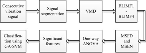
Variational mode decomposition (VMD) was recently proposed by Konstantin D. and Dominique Z. [19]. It is a new adaptive signal decomposition method which can adaptively determine the relevant frequency bands and the corresponding mode simultaneously. In other words, VMD has the capability of decomposing an arbitrary signal into a series of band-limited intrinsic mode functions (BLIMFs). The VMD algorithm has solid theoretical foundation, its substance is several adaptive wiener filtering and it also shows better noise robustness. Wang et al. [20] had already adopted the VMD to analyze the rubbing signals and concluded that the multiple features can be better extracted using VMD than EMD and EEMD. We thus employed VMD to decompose the vibration signal in this paper, and then adopted the multiscale fractal dimension (MSFD) and multiscale energy (MSEN) to extract features. In an attempt to improve the classification speed, the one-way analysis of variance (ANOVA) test was adopted to remove the redundant features and the remaining significant features were bound together to constitute the feature vectors of vibration signals. After the procedure of feature extraction for the vibration signals, a multi-fault classifier should be applied to recognize the fault mode. As one of the most state-of-the-art and popular classifiers, support vector machine (SVM) [21] demonstrates many specific advantages in solving small samples, nonlinear and high-dimension pattern recognition problems. Whereas, the choice of appropriate parameters of SVM was difficult, therefore SVM optimized by the genetic algorithm (GA), i.e., GA-SVM was exploited as the multi-fault classifier in the current study. The block diagram of the proposed method is presented in Fig. 1.

The rest of this paper is organized as follows. Section 2 gives the detailed description about the vibration signal data we used. Section 3 introduces the principle of the new time-frequency analysis method-VMD, the algorithm of MSFD and MSEN as well as the mechanism of GA-SVM. Experimental results are presented in Section 4. Finally, conclusions are drawn in Section 5.

Fig. 1Concrete process of the proposed method

2. Rolling bearing database

To verify the effectiveness of the proposed method in this study, a public vibration signal dataset, obtained from the Case Western Reserve University bearing data center website, was employed [22]. The test data collection device and description were given in detail in [22]. The 6205-2RS JEM SKF deep groove ball bearings were used in the test as the testing bearings. The test bearings support the motor shaft, single point faults were introduced to test bearings using electro-discharge machining with fault diameters of 0.1778 mm and 0.3556 mm, both with the same fault depth. Vibration data was collected by accelerometers, which were attached to the housing with magnetic bases. And the data we used in this work was collected through accelerometers which were placed at the 12 o’clock position at drive end of the motor housing. The sampling frequency of the vibration data was 12000 Hz.

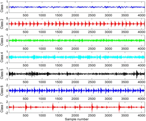
In our study, the database was divided into seven subsets. With motor load changed from 0 to 3 horsepower (motor speeds of 1797 RPM to 1720 RPM ), the subset 1 was the collection of vibration signal in normal condition; the subsets 2 and 3 were taken from the outer race fault, whose fault diameter were 0.1778 mm and 0.3556 mm, respectively; the subsets 4 and 5 were measured from the ball element fault, whose diameter fault were 0.1778 mm and 0.3556 mm, respectively; the remaining subsets 6 and 7 were derived from the inner race fault, whose diameter fault were 0.1778 mm and 0.3556 mm, respectively. Our objective was to identify the seven statuses, namely normal, outer race fault 1, outer race fault 2, ball element fault 1, ball element fault 2, inner race fault 1 and inner race fault 2 automatically and accurately. To achieve this aim, the continuous sequence of each subset was segmented into isometric samples with a length of 4096. As a consequence, for each kind of the subset, the obtained number of samples was 116. Among them, 58 samples were randomly selected as training set and the remaining samples were used as testing set. A detailed description of the segmented vibration signals is shown in Table 1 and the time domain waveforms of these seven classes of rolling bearing vibration signals are shown in Fig. 2.

Table 1A detailed description about the vibration signal

Database	Rolling bearing fault	Defect size (mm)	Class	Data distribution
Database	Rolling bearing fault	Defect size (mm)	Class	Training samples	Testing samples	Total samples
Subset 1	Normal	0	1	58	58	116
Subset 2	Outer race 1	0.1778	2	58	58	116
Subset 3	Outer race 2	0.3556	3	58	58	116
Subset 4	Ball element 1	0.1778	4	58	58	116
Subset 5	Ball element 2	0.3556	5	58	58	116
Subset 6	Inner race 1	0.1778	6	58	58	116
Subset 7	Inner race 2	0.3556	7	58	58	116

3. Methodology

This section is composed of three subsections: the principle of VMD is presented in the first subsection; subsequently, the MSFD and MSEN are proposed in the second subsection; finally, the optimized SVM, i.e., GA-SVM is introduced in the last subsection.

Fig. 2Typical waveform of seven classes of rolling bearing vibration signals

3.1. Variational mode decomposition

VMD is a newly-developed method for adaptive and quasi-orthogonal signal decomposition, and it is very robust against noise and sampling [19]. VMD is able to decompose a real valued signal $f$ into a discrete number of sub-signals $u_{k}$ . Each sub-signal, namely BLIMF, has specific sparsity properties while reproducing the input [19]. Here, each mode $u_{k}$ should be mostly compacted around a center pulsation $w_{k}$ . The proposition of VMD can be summarized as a constrained variational problem [19]:

1

\{\begin{array}{l} \underset{{u_{k}}, {w_{k}}}{m i n} \{\sum_{k} {‖\partial_{t} [(δ (t) + \frac{j}{π t}) * u_{k} (t)] e^{- j w_{k} t} |‖}_{2}^{2}\} . \\ s . t . \sum_{k = 1} u_{k} = f \end{array}

To solve Eq. (1), the quadratic penalty term and Lagrangian multipliers $λ$ are introduced. Accordingly, the augmented Lagrangian is given as following [19]:

2

L ({u_{k}}, {w_{k}}, λ) = α \sum_{k} {‖\partial_{t} [(δ (t) + \frac{j}{π t}) * u_{k} (t) e^{- j w_{k} t}]‖}_{2}^{2}

+ {‖f (t) - \sum_{k} u_{k} (t)‖}^{2} + 〈λ (t), f (t) - \sum_{k} u_{k} (t)〉,

where $α$ represents the balance parameter of the data fidelity.

The alternate direction method of multipliers (ADMM) [23] is introduced to solve the augmented Lagrangian problem. By alternating renewal $u_{k}^{n + 1}$ , $w_{k}^{n + 1}$ , $λ^{n + 1}$ to search the saddle point of the extend Lagrangian expression. In this case, the value of $u_{k}^{n + 1}$ can be described as:

3

u_{k}^{n + 1} = \underset{u_{k} \in X}{a r g m i n} \{α {‖\partial_{t} [(δ (t) + \frac{j}{π t}) * u_{k} (t)] e^{- j w_{k} t}‖}_{2}^{2} + {‖f (t) - \sum_{i} u_{i} (t) + \frac{λ (t)}{2}‖}_{2}^{2}\} .

According to Parseval/Plancherel Fourier isometric transformation, the frequency-domain expression of Eq. (3) can be expressed as [19]:

4

{\hat{u}}_{k}^{n + 1} = \underset{{\hat{u}}_{k}, u_{k} \in X}{a r g m i n} {α {‖j w [(1 + s g n (w + w_{k})) \cdot {\hat{u}}_{k} (w + w_{k})]‖}_{2}^{2}

+ {‖\hat{f} (w) - \sum_{i} {\hat{u}}_{i} (w) + \frac{\hat{λ} (w)}{2}‖}_{2}^{2} .

By means of a series of computation, solution of the quadratic optimization issue is given by [19]:

5

{\hat{u}}_{k}^{n + 1} (w) = \frac{\hat{f} (w) - \sum_{i \neq k} {\hat{u}}_{i} (w) + \frac{\hat{λ} (w)}{2}}{1 + 2 α (w - w_{k})^{2}} .

According to the same process, the recursion formula of the center frequency is obtained as [19]:

6

w_{k}^{n + 1} = \frac{\int_{0}^{\infty} w | {\hat{u}}_{k} (w) |^{2} d w}{\int_{0}^{\infty} | {\hat{u}}_{k} (w) |^{2} d w} .

By implementing VMD, the raw vibration signal is decomposed into a fixed number of subcomponents (BLIMFs). Under the circumstances, the hidden characteristics of vibration signals are revealed and feature extraction procedure is subsequently carried out.

3.2. Multiscale fractal dimension and energy

Fractal dimensions (FD) can quantitatively characterize the non-linear behavior of the vibration signals. There are many computing methods of FD, such as box-counting dimension, information dimension, correlation dimension, similar dimension, spectral dimension and so forth. Among them, the box-counting dimension [24] is widely used because of its easier calculation method compared with other methods. Therefore, the box-counting dimension is applied to quantify the nonlinear characteristic of BLIMFs in this paper.

For a given discrete sequence ${x (j), j = 1,2, . . ., N_{0}}$ and $x$ is the closed set of $n$ dimension geometry space $R^{n}$ . $R^{n}$ is divided into as many grids as possible. The width of the grid is $Δ$ , $Δ$ is defined as the smallest grid and being multiplied by positive integer $m$ defined as $m Δ$ , $N_{m Δ}$ is the box counting number in the discrete signal $X$ with the grid which the width is $m Δ$ . Suppose $P (m Δ)$ is the scope of longitudinal coordinate and $N_{m Δ}$ is the corresponding box counting number, and they can be calculated as follows [24]:

7

\{\begin{array}{l} P (m Δ) = (\begin{matrix} \sum_{j = 1}^{N_{0} / m} | m a x {x_{m (j - 1) + 1}, x_{m (j - 1) + 2}, \dots, x_{m (j - 1) + m + 1}} \\ - m i n {x_{m (j - 1) + 1}, x_{m (j - 1) + 2}, \dots, x_{m (j - 1) + m + 1}} | \end{matrix}), \\ N_{m Δ} = \frac{P (m Δ)}{m Δ} + 1, j = 1,2, 3, . . ., \frac{N_{0}}{m}, m = 1,2, . . ., M, M < N_{0} . \end{array}

The scale-less region is defined as the scope within the line with good linearity in the coordinate system of $l g m Δ ~ l g N_{m Δ}$ . The start point and end point of the scale-less region are defined as $m_{1}$ , $m_{2}$ , then least square is adopted to fit the linear variation trend. The estimated value of the slope of the fitting line is regarded as the value of box-counting dimension [24]:

8

d_{B} = - \frac{(m_{2} - m_{1} + 1) \sum l g m l g N_{m Δ} - \sum l g m \sum l g N_{m Δ}}{(m_{2} - m_{1} + 1) \sum l g^{2} m - (\sum l g m)^{2}}, m_{1} \leq m \leq m_{2} .

Energy can reflect the energy distribution property of each BLIMF and it is beneficial for recognizing different rolling bearing fault categories. Given this, the energy of each BLIMF is calculated. In our study, energy is defined as the sum of the absolute value of signal and it is given by:

9

E n = \sum_{n} |x (n)|,

where $n$ is the number of sampling points.

By extracting the box-counting dimension and energy, the redundant time-domain signal has been condensed into a two-dimensional feature vector. However, a single scale fractal dimension and energy only provide the global information. To reveal more comprehensive characteristics of a signal, multiscale [25] is introduced. MSFD and MSEN are the extensional versions of conventional fractal dimension and energy, which describe the characteristics of the experimental objects under different scale factors.

The procedure of MSFD and MSEN consist of two steps: (1) coarse-grained operation and (2) calculating FD/Energy using coarse-grained vector. Concretely, for a one-dimensional data series $x$ of $N$ sampling points, the new coarse-grained vector can be constructed as:

10

y_{j}^{τ} = \frac{1}{τ} \sum_{i = (j - 1) τ + 1}^{j τ} x_{i}, 1 \leq j \leq ⌊\frac{N}{τ}⌋ .

Fig. 3The coarse grained vector under different scale factors

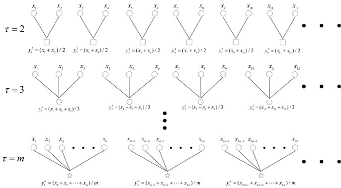
In this case, different value of $τ$ can produce different coarse-grained vector, and then its corresponding fractal dimension and energy can be calculated. When $τ$ equals to one, the coarse grained vector becomes the original time series $x$ ; on the other hand, if $τ$ is greater than one, the original data is divided into $N / τ$ coarse grained vector ${y^{τ}}$ (shown in Fig. 3). Based on above presented principle of multiscale analysis, the MSFD and MSEN of each BLIMF are calculated as features of the raw vibration signals.

3.3. Support vector machine

SVM, which is structured based on Vapnik-Chervonenkis (VC) dimension theory and structural risk minimization (SRM) rule, was firstly proposed by Vapnik et al. [26]. As one of the state-of-the-art machine learning algorithms, SVM shows many specific advantages in solving small sample, non-linear and high-dimension pattern recognition problems [27].

For $N$ training samples ${(x_{1}, y_{1}), (x_{2}, y_{2}), \dots (x_{N}, y_{N})}$ , where the $i$ th sample $x_{i} \in R^{n}$ and it belongs to one label $y_{i} =$ +1 or $y_{i} =$ –1. Where +1 and –1 represent the positive and negative classes respectively. By mapping the input vector $x$ into the higher-dimensional feature space, the linearly separable hyperplane is defined as [26]:

11

ω \cdot x + b = 0,

where $ω$ is the hyperplane’s normal vector, and $b$ is a constant.

When the inputs are linearly inseparable, slack variable $ξ_{i}$ is introduced. Accordingly, the issue of constructing optimal hyperplane is translated into a constraint equation [26]:

12

\{\begin{array}{l} m i n \frac{1}{2} {‖ω‖}^{2} + C \sum_{i = 1}^{N} ξ_{i}, \\ s . t . y_{i} (ω \cdot ϕ (x) + b) - 1 + ξ_{i} \geq 0, ξ_{i} \geq 0, i = 1,2 . . . ., N, \end{array}

where $C$ represents the penalty parameter and $ϕ$ is a mapping function which responsible for mapping the inputs into a higher-dimensional feature space.

To solve the above-mentioned optimization issue, Lagrange multipliers are introduced and Eq. (13) is rewritten as [26]:

13

\begin{array}{l} m a x \sum_{i = 1}^{N} α_{i} - \frac{1}{2} \sum_{i = 1}^{N} α_{i} α_{j} y_{i} y_{j} K (x_{i}, x_{j}), \\ s . t . \sum_{i = 1}^{M} α_{i} y_{i} = 0, α_{i} \geq 0, i = 1,2, \dots, N, \end{array}

where $K (x_{i}, x_{j}) = ϕ (x_{i}) \cdot ϕ (x_{j})$ is the kernel function of SVM, $α_{i}$ is the Lagrange multiplier.

Eventually, the optimal classification function can be obtained as [26]:

14

f (x) = s g n (\sum_{i = 1}^{N} α_{i} y_{i} K (x_{i}, x) + b)) .

There are multiple kernel functions, the linear, polynomial and radial basis function (RBF) kernel functions are the popular ones [27]. Among them, RBF kernel is the most widely used kernel function and it is adopted in this work. The expression of RBF is given by:

15

K (x, x_{i}) = e x p (- \frac{{‖x - x_{i}‖}^{2}}{2 σ^{2}}) .

It should be emphasized that SVM is substantially a binary classifier, while in this paper our objective is to classify seven kinds of rolling bearing vibration signals. Up until now, various algorithms have been presented to structure the multi-class SVM. Among them, the one-versus-rest (OVR) [26], one-versus-one (OVO) [28] and directed acyclic graphs (DAG) [29] are the most common used approaches. In the presented study, the OVO technique is selected to construct the multi-class SVM for differentiating seven types of vibration signals. In OVO, a child classification model is built on any two groups of training samples. Therefore, for a $k$ -classifying case, $k \times (k - 1) / 2$ binary child classifiers are required, that is, 21 SVMs are utilized to establish the seven-classifying SVM classifier. When a testing sample is fed into the established classifier for classification, its final class is the label which gains the most votes.

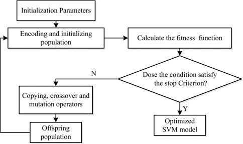
Additionally, penalty parameter $C$ and kernel parameter $σ$ play a crucial role in determining the classification performance of SVM [30]. Given this, GA [30] is applied to search for the best combination of parameters $C$ and $σ$ . The main parameters of GA are the generations, population size, crossover probability and mutation probability. In our study, the generations, population size, crossover probability and mutation probability are set to 200, 20, 0.9 and 0.05, respectively. Furthermore, the value ranges of $C$ and $σ$ are both set to the range of 0.1 to 200. A brief flowchart of optimizing SVM using GA is illustrated in Fig. 4.

Fig. 4Flowchart of optimizing SVM using GA

4. Results

In current paper, all experiments were implemented in MATLAB 2013a environment and a 2.53 GHz Core^TM processor. In this section, the experimental results of extracting BLIMFs using VMD are presented in the first part, and then the calculated MSFD and MSEN of each BLIMF are presented in the second part. Subsequently, one-way ANOVA test was implemented and the features were ranked according their $F$ -value, then those significant features were selected and fed into a GA-SVM for classification. Finally, the classification performance under different signal-to-noise ratios (SNRs) was discussed.

4.1. Waveform extraction based on VMD

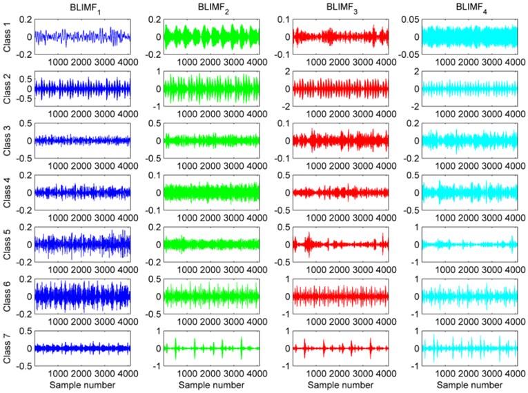
The VMD algorithm is able to decompose an arbitrary signal into a series of BLIMFs. Before implementing VMD, we should give the mode number $k$ , different center frequencies could be useful in distinguishing kinds of patterns. After many experiments, we found that when $k =$ 4, the center frequencies were diverse from each other. As a consequence, the number of BLIMFs was set to 4. Each rolling bearing class had 58 training samples, we selected one sample as the experimental subject to show the results of VMD. The four corresponding BLIMFs of these seven kinds of vibration signals are shown in Fig. 5. As illustrated in Fig. 5, each BLIMF of these seven classes of vibration signals somewhat varies from each other. Concretely speaking, the most obvious characteristic is each BLIMF of Class 2, 6 and BLIMF₂ to BLIMF₄ of Class 7 contains distinct impulse component but others not or not so obvious. Moreover, the main energy concentrations of Class 1, 2, 3, 4, 5, 6, 7 are in BLIMF₂, BLIMF₃/BLIMF₄, BLIMF₂, BLIMF₄, BLIMF₃/BLIMF₄, BLIMF₃/BLIMF₄, BLIMF₂/BLIMF₃/ BLIMF₄, respectively. There is no doubt that these waveforms are different from each other, however, it is still a very hard work to identify the fault mode from the extracted waveforms.

Fig. 5Plots of BLIMFS after decomposing the seven classes of vibration signal based on the VMD

4.2. Feature extraction based on MSFD and MSEN

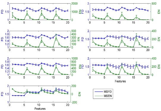
Each kind of vibration signals had been decomposed into four BLIMFs after applying VMD. In an attempt to extract features of BLIMFs of rolling bearing segments, we computed the MSFD and MSEN of four generated BLIMFs as the condensed features, and this procedure was known as feature extraction. In this section, we gave the mean value and standard deviation of MSFD and MSEN of each BLIMF of the 58 samples of each class in Fig. 6. For each kind of vibration signals, which had four decomposed BLIMFs, the 5-scale MSFD and MSEN of each BLIMF were computed, and then they were arranged into a 40-dimension feature vectors. The horizontal axis represents the features, among them, the first five features represent the 5-scale features of BLIMF₁, the 6-10 features mean the 5-scale features of BLIMF₂, the 11-15 and 16-20 features represent the 5-scale features of BLIMF₃ and BLIMF₄, respectively. The blue and green lines stand for the statistics trend of MSFD and MSEN of these four BLIMFs. The error bar in the plot shows the magnitude of the standard deviation, and the middle of the error bar is the mean value of MSFD and MSEN. The first row of this figure shows results of outer race1 (left subgraph) and outer race 2 (right subgraph); the second row exhibits the results of ball element 1 (left subgraph) and ball element 2 (right subgraph); the third row displays the results of inner race 1 (left subgraph) and inner race 2 (right subgraph) and the fourth row, namely, the last subgraph, is the results of the normal condition of the rolling bearing.

From Fig. 6, it can be observed that the MSFD and MSFN of the normal condition of the rolling bearing change a little and keep smoothly. Furthermore, their error bars are smaller than others’, and the mean MSEN fluctuates near zero. In addition, the 5-scale MSFD of BLIMF₁ are almost the same, which indicates that the vibration signals of the normal condition are steady. Considering the maximum peaks of MSEN for other fault conditions, the values of outer race 1, ball element 1 and inner race 1 are close to 1000, 300 and 600, respectively. The variation range of MSFD of outer race fault is the biggest one among all the faults; on the contrary, the range of MSFD of inner race fault is the smallest. For the outer race fault, the error bars of outer race 1 are longer than that of outer race 2, and it indicates that the greater the damage, the shorter error bars obtained. What’s more, the maximum peak of the MSEN of outer race 1 is bigger than that of outer race 2. For the ball element and inner race fault, the greater the damage, the longer the error bars shown, as well as the smaller maximum peak of the MSEN measured.

Fig. 6The mean value and standard deviation of MSFD and MSEN

4.3. Classification using GA-SVM

We had extracted 20-dimensional MSFD and 20-dimensional MSEN features after applied multiscale analysis. Among the 40-dimensional features, some features were redundant and they contributed few for classification accuracy. In order to obtain the significant features and reduce the computational complexity, we employed the one-way ANOVA test to analyze each feature, and then we could get the $F$ -statistic values corresponding to each feature. The $F$ -value represents the significance level, the larger the value of $F$ , the more significance level is. Hence we could conclude that a large $F$ leaded to a high classification accuracy in some degree. Fig. 7 shows the result of carrying out one-way ANOVA for each feature, and the first 20-dimensional features represent the $F$ value of MSFN, and the last 20-dimensional features signify the $F$ value of MSEN. Through the presented histogram of $F$ , we could easily distinguish which feature made more contribution to the classification performance. For example, the second dimensional feature has the greatest $F$ -value and it indicates that the second dimensional feature possesses the greatest impact on classification accuracy. On the contrary, the $F$ -value of 24th dimensional feature is smallest, which imply that the 24th dimensional feature is likely to be redundant and has tiny influence on classification performance.

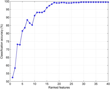
Rearranged the order of the 40-dimensional features according to the $F$ -value from largest to smallest. In this case, the first ranked feature possesses the largest $F$ and the last ranged feature owns the smallest $F$ . Subsequently, 40 times independent experiments were implemented for various cases. For the $m$ th ( $m =$ 1, 2,..., 40) experiment, the first m-dimensional features were fed into the GA-SVM for classification, respectively. In addition, in order to guarantee the stability and veracity of classification accuracy, 10-fold cross validation was also adopted in the classification step and final classification accuracy was obtained and shown in Fig. 8. From Fig. 8, we know that along with the increase of the number of employed features, the classification accuracy is maintaining growth. When the number of feature dimensions increased to 30, the classification accuracy reaches a maximum value, and the classification accuracy no longer or barely changed with the increase of the feature dimensions. Therefore we could concluded that the first ranked 30-dimensional features could best represent the difference of the seven classes rolling bearing statuses under the premise of ensuring high accuracy, and the last 10-dimension features were redundant and they contributed a little for classification performance, thus we eliminated the last 10-dimension features and just employed the first 30-dimension features as the significant features to distinguish the seven classes rolling bearing statuses.

By applying one-way ANOVA test, we had extracted the significant features from the redundant features. Subsequently, the training samples were used to build the GA-SVM classifier. Once again, the 10-fold cross validation was utilized to prevent overfitting and obtain the appropriate parameters of SVM in training procedure. Finally, the remaining testing samples were fed into the trained GA-SVM to verify the rationality of the established classifier, and the predicted categories of testing samples are shown in Fig. 9. As displayed in Fig. 9, only one sample is misclassified among the 406 testing samples, and the classification accuracy is as high as 99.75 %.

Fig. 7Results of one-way ANOVA for each feature

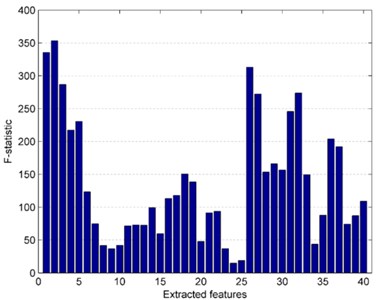
Fig. 8Classification accuracy of the ranked feature in 40 cases

In an attempt to prove the necessity of decomposing the original signals, in addition to above experiment, we also calculated the MSFD and MSEN of the original signals directly, and then the extracted feature vectors were used to train and test the newly-built GA-SVM classifier. The rolling bearing data used in the experiment was the same as above-mentioned data and the final classification result without decomposing the vibration signals is shown in Fig. 10. As illustrated in Fig. 10, there exists 9 misclassified samples among the 406 testing samples, and the classification accuracy was 97.78 %. Compared with Fig. 9, this result indicates that it is necessary to decompose the original vibration signal using VMD before extracting features from the original vibration signals.

4.4. Influence of noise on classification performance

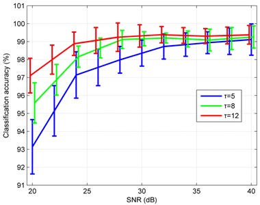
In practical situations, the collected vibration signals are inevitably contaminated by noise. It is necessary to investigate the anti-noise property of the presented diagnosis method in different signal-to-noise ratio (SNR). Besides, with the decline of SNR, a 5-scale feature extraction operation might result in mediocre classification accuracy and a higher-scale operation should be taken into account. Hence, to simulate actual situations, the Gaussian white noise at diverse levels was added in the original signals and three different scales, namely 5-, 8- and 12-scale feature extraction operations were studied. Fig. 11 plots the error bars of the classification accuracy under different scales and SNRs. As shown in Fig. 11, a phenomenon can be observed that the larger the scale is, the higher classification accuracy can be achieved. Given a specified multiscale value, with the increase of SNR, the classification accuracy becomes higher and higher. When SNR is less than 30 dB, a higher-scales operation should be chosen to acquire the better classification accuracy. While SNR is larger than 30 dB, the lower-scales can lead to an approving classification accuracy with a faster computing speed.

Fig. 9Classification results of the earlier 30-dimension features

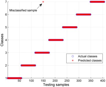
Fig. 10Classification results without decomposing the original vibration signals

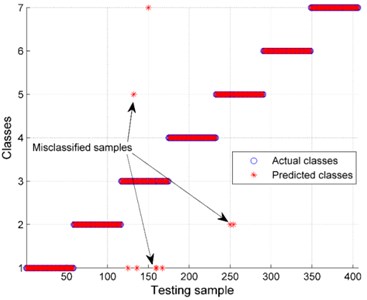
Fig. 11Classification performances of GA-SVM with the variation of SNRs and scales

5. Conclusions

In this paper, we proposed a novel rolling bearing fault diagnosis method based on VMD-multiscale fractal dimension/energy and GA-SVM. Seven classes of rolling bearing vibration signals were used to verify the effectiveness of the proposed method and the classification accuracy is as high as 99.75 %. In addition, our approach shows good anti-noise performance in different signal-to-noise ratios. The method we proposed can be a useful tool to monitor the rolling bearing operating state automatically and accurately. It can assist the rotating machinery users detect the fault degree and fault location timely and avoid the unnecessary downtime of the rotating machinery, the reliability of the rotating machinery can thus be improved. Future directions of our research may include application of the proposed method for diagnosis of other mechanical faults.

References

Li M., Wang M., Wang C. G. Research on SVM classification performance in rolling bearing diagnosis. International Conference on Intelligent Computation Technology and Automation, 2010, p. 132-135.

Search CrossRef
Logan D., Mathew J. Using the correlation dimension for vibration fault diagnosis of rolling element bearings. Part 1: basic concepts. Mechanical Systems and Signal Processing, Vol. 10, Issue 3, 1996, p. 241-250.

Publisher
Zhang P. L., Li B., Mi S. S. Bearing fault detection using multiscale fractal dimensions based on morphological covers. Shock and Vibration, Vol. 19, Issue 6, 2012, p. 1373-1383.

Publisher
Yan R., Gao R. X. Approximate Entropy as a diagnostic tool for machine health monitoring. Mechanical Systems and Signal Processing, Vol. 21, Issue 2, 2007, p. 824-839.

Publisher
Wang F., Zhang Y., Zhang B. Application of wavelet packet sample entropy in the forecast of rolling element bearing fault trend. International Conference on Multimedia and Signal Processing, IEEE Computer Society, 2011, p. 12-16.

Publisher
Liu H., Han M. A fault diagnosis method based on local mean decomposition and multiscale entropy for roller bearings. Mechanism and Machine Theory, Vol. 75, Issue 5, 2014, p. 67-78.

Publisher
Chen W., Wang Z., Xie H. Characterization of surface EMG signal based on fuzzy entropy. IEEE Transactions on Neural Systems and Rehabilitation Engineering, Vol. 15, Issue 2, 2007, p. 266-272.

Publisher
Zheng J., Cheng J., Yang Y. A rolling bearing fault diagnosis method based on multiscale fuzzy entropy and variable predictive model-based class discrimination. Mechanism and Machine Theory, Vol. 78, Issue 16, 2014, p. 187-200.

Publisher
Tse P. W., Peng Y. H., Yam R. Wavelet analysis and envelope detection for rolling element bearing fault diagnosis – their effectiveness and flexibilities. Journal of Vibration and Acoustics, Vol. 123, Issue 3, 2001, p. 303-310.

Publisher
Kankar P. K., Sharma S. C., Harsha S. P. Rolling element bearing fault diagnosis using wavelet transform. Neurocomputing, Vol. 74, Issue 10, 2011, p. 1638-1645.

Publisher
Zhong X. Y., Zhao C. H., Dong H. J., Liu X. M., Zeng L. C. Rolling bearing fault diagnosis using sample entropy and 1.5-dimension spectrum based on EMD. Applied Mechanics and Materials, 2013, p. 1027-1031.

Publisher
Zhao S. F., Liang L., Xu G. H. Quantitative diagnosis of a spall-like fault of a rolling element bearing by empirical mode decomposition and the approximate entropy method. Mechanical Systems and Signal Processing, Vol. 40, Issue 1, 2013, p. 154-177.

Publisher
Zhu K., Song X., Xue D. Incipient fault diagnosis of roller bearings using empirical mode decomposition and correlation coefficient. Journal of Vibroengineering, Vol. 15, Issue 2, 2009, p. 597-603.

Search CrossRef
Smith J. S. The local mean decomposition and its application to EEG perception data. Journal of the Royal Society Interface, Vol. 2, Issue 5, 2005, p. 443-454.

Publisher
Cheng J., Yang Y., Yang Y. A rotating machinery fault diagnosis method based on local mean decomposition. Digital Signal Processing, Vol. 22, Issue 2, 2012, p. 356-366.

Publisher
Mark G. Frei Intrinsic time-scale decomposition: time-frequency-energy analysis and real-time filtering of non-stationary signals. Royal Society of London Proceedings, Vol. 463, Issue 2078, 2007, p. 321-342.

Publisher
Luo S. R., Cheng J. S., Zheng J. D. Early fault diagnosis of rolling bearing based on ITD fractal fuzzy entropy. Journal of Vibration, Measurement and Diagnosis, Vol. 33, Issue 4, 2013, p. 706-711.

Search CrossRef
Zheng J., Cheng J., Yang Y. A rolling bearing fault diagnosis approach based on LCD and fuzzy entropy. Mechanism and Machine Theory, Vol. 70, Issue 6, 2013, p. 441-453.

Publisher
Konstantin D., Dominique Z. Variational mode decomposition. IEEE Transactions on Signal Processing, Vol. 3, Issue 62, 2014, p. 531-544.

Publisher
Wang Y., Markert R., Xiang J. Research on variational mode decomposition and its application in detecting rub-impact fault of the rotor system. Mechanical Systems and Signal Processing, Vol. 60, 2015, p. 243-251.

Publisher
Li X., Zheng A., Zhang X. Rolling element bearing fault detection using support vector machine with improved ant colony optimization. Measurement, Vol. 46, Issue 8, 2013, p. 2726-2734.

Publisher
Loparo K. A. Bearings Data Center. Case Western Reserve University, http://csegroups.case.edu/bearingdatacenter/home.

Search CrossRef
Tosserams S., Etman L. F. P., Papalambros P. Y. An augmented Lagrangian relaxation for analytical target cascading using the alternating direction method of multipliers. Structural and Multidisciplinary Optimization, Vol. 31, Issue 3, 2006, p. 176-189.

Publisher
Yang G., Liu Y., Zhao L. Typical power quality disturbance identification based on fractal box dimension. International Workshop on Chaos-Fractals Theories and Applications, 2009, p. 412-416.

Publisher
Costa M. Multiscale entropy analysis of complex physiologic time series. Physical Review Letters, Vol. 89, Issue 3, 2002, p. 705-708.

Publisher
Vapnik V. N. The Nature of Statistical Learning Theory. Springer-Verlag, New York, 1995.

Publisher
Yang J., Zhang Y., Zhu Y. Intelligent fault diagnosis of rolling element bearing based on SVMs and fractal dimension. Mechanical Systems and Signal Processing, Vol. 21, Issue 5, 2007, p. 2012-2014.

Publisher
Knerr S., Personnaz L., Dreyfus G. Single-layer learning revisited: a stepwise procedure for building and training a neural network. Neurocomputing, Vol. 68, 1990, p. 41-50.

Publisher
Platt J. C., Cristianini N., Shawe-Taylor J. Large margin DAGs for multiclass classification. Advances in Neural Information Processing Systems, Vol. 12, Issue 3, 2000, p. 47-553.

Search CrossRef
Sajan K. S., Kumar V., Tyagi B. Genetic algorithm based support vector machine for on-line voltage stability monitoring. International Journal of Electrical Power and Energy Systems, Vol. 75, 2015, p. 200-208.

Publisher

Cited by

A novel motor fault diagnosis method based on principal component analysis (PCA) with a discrete belief rule base (DBRB) system

Hang Yu | Haibo Gao | Yelan He | Zhiguo Lin | Xiaobin Xu

(2023)

Imbalanced fault classification of rolling bearing based on an improved oversampling method

Yanfang Han | Baozhu Li | Yingkun Huang | Liang Li | Kang Yan

(2023)

Short-Term Power Prediction by Using Least Square Support Vector Machine With Variational Mode Decomposition in a Photovoltaic System

(2023)

A Novel Multiple Feature-Based Engine Knock Detection System using Sparse Bayesian Extreme Learning Machine

(2022)

Minimization of the vestigial noise problem of empirical wavelet transform to detect bearing faults under time-varying speeds

Vikas Sharma | Pradeep Kundu

(2022)

The Fault Diagnosis of Rolling Bearing Based on Improved Deep Forest

(2021)

About this article

Received

18 January 2016

Accepted

08 August 2016

Published

30 September 2016

SUBJECTS

Fault diagnosis based on vibration signal analysis

DOI

https://doi.org/10.21595/jve.2016.16847

Keywords

rolling bearing fault diagnosis

variational mode decomposition (VMD)

multiscale fractal dimension (MSFD)

multiscale energy (MSEN)

support vector machine (SVM)

Acknowledgements

This work is supported by the Specialized Research Fund of the One Thousand sets of Domestic CNC Lathe Reliability Engineering (Grant No. 2013ZX04011-011).

Author Contributions

Fei Chen conceived the idea of using vibration data to identify the rolling bearing fault and guide the writing of the whole paper. Xiaojuan Chen conducted the method to better identify the various rolling beading fault modes and wrote the majority of the paper. Zhaojun Yang studied the application of the method VMD and apply it to our paper. Binbin Xu chosen the experimental data and analyzed the results. Qunya Xie made the procedure of the optimized SVM and obtained the value of the corresponding parameters. Heng Zhang read a lot of literatures and wrote the Instructions. Yifeng Ye edited the manuscript and checked the grammatical and spelling errors.

This is an open access article distributed under the Creative Commons Attribution License, which permits unrestricted use, distribution, and reproduction in any medium, provided the original work is properly cited.

Previous article in issue Previous Next article in issue Next

Research article

2024 01 21

Rolling bearing fault diagnosis based on variational mode decomposition and weighted multidimensional feature entropy fusion

Na Lei, Feihu Huang, Chunhui Li

Research article

2023 09 08

Research on fault diagnosis method of bearing based on parameter optimization VMD and improved DBN

Yingqian Sun, Zhenzhen Jin

Research article

2023 08 01

Motor rolling bearing fault diagnosis based on MVMD energy entropy and GWO-SVM

Jian Tang, Qiaoni Zhao

Research article

2022 12 18

Fault feature extraction method for rolling bearing based on MVMD and complex Fourier transform

Chuanjin Huang, Haijun Song

F. Chen et al., “A rolling bearing fault diagnosis method based on VMD – multiscale fractal dimension/energy and optimized support vector machine,” Journal of Vibroengineering, Vol. 18, No. 6, pp. 3581–3595, Sep. 2016, https://doi.org/10.21595/jve.2016.16847

Copy Extrica

Copied to clipboard!

TY  - JOUR
DO  - 10.21595/jve.2016.16847
UR  - https://doi.org/10.21595/jve.2016.16847
TI  - A rolling bearing fault diagnosis method based on VMD – multiscale fractal dimension/energy and optimized support vector machine
T2  - Journal of Vibroengineering
AU  - Xu, Binbin
AU  - Chen, Fei
AU  - Chen, Xiaojuan
AU  - Yang, Zhaojun
AU  - Xie, Qunya
AU  - Zhang, Heng
AU  - Ye, Yifeng
PY  - 2016
DA  - 2016/09/30
PB  - JVE International Ltd.
SP  - 3581-3595
IS  - 6
VL  - 18
SN  - 1392-8716
ER  - 

Copy Ris

Copied to clipboard!

@article{Xu_2016,
	doi = {10.21595/jve.2016.16847},
	url = {https://doi.org/10.21595/jve.2016.16847},
	year = 2016,
	month = {sep},
	publisher = {{JVE} International Ltd.},
	volume = {18},
	number = {6},
	pages = {3581--3595},
	author = {Binbin Xu and Fei Chen and Xiaojuan Chen and Zhaojun Yang and Qunya Xie and Heng Zhang and Yifeng Ye},
	title = {A rolling bearing fault diagnosis method based on {VMD} {\textendash} multiscale fractal dimension/energy and optimized support vector machine},
	journal = {Journal of Vibroengineering}
}

Copy Bibtex

Copied to clipboard!

[1]B. Xu et al., “A rolling bearing fault diagnosis method based on VMD – multiscale fractal dimension/energy and optimized support vector machine,” Journal of Vibroengineering, vol. 18, no. 6, pp. 3581–3595, Sep. 2016, doi: 10.21595/jve.2016.16847.

Copy IEEE

Copied to clipboard!

Xu, Binbin, Fei Chen, Xiaojuan Chen, Zhaojun Yang, Qunya Xie, Heng Zhang, and Yifeng Ye. “A Rolling Bearing Fault Diagnosis Method Based on VMD – Multiscale Fractal Dimension/Energy and Optimized Support Vector Machine.” Journal of Vibroengineering 18, no. 6 (September 30, 2016): 3581–95. https://doi.org/10.21595/jve.2016.16847.

Copy Chicago

Copied to clipboard!

A rolling bearing fault diagnosis method based on VMD – multiscale fractal dimension/energy and optimized support vector machine

Abstract

1. Introduction

2. Rolling bearing database

3. Methodology

3.1. Variational mode decomposition

3.2. Multiscale fractal dimension and energy

3.3. Support vector machine

4. Results

4.1. Waveform extraction based on VMD

4.2. Feature extraction based on MSFD and MSEN

4.3. Classification using GA-SVM

4.4. Influence of noise on classification performance

5. Conclusions

References

Cited by

About this article

Related Articles