The analysis of vortex induced vibration of the flexible pipe in a cylindrical fluid field with cross flow

Liu, Ju-Bao; Yue, Qian-Bei; Dong, Ri-Zhi; Zhang, Qiang

doi:10.21595/jve.2016.16547

Journal of Vibroengineering

Browse Journal

Submit article

Published: 30 June 2016

Check for updates

The analysis of vortex induced vibration of the flexible pipe in a cylindrical fluid field with cross flow

Ju-Bao Liu¹

Qian-Bei Yue²

Ri-Zhi Dong³

Qiang Zhang⁴

^{1, 2, 3, 4}College Mechanical Science Engineering, Northeast Petroleum University, Hei Long-Jiang, Daqing 163318, China

Corresponding Author:

Qian-Bei Yue

Cite the article Download PDF

Downloads 1903

Abstract

In view of the vortex-induced vibration of the flexible pipe in the limited fluid domain, the flexible pipe was dispersed into several three-dimensional beam elements and the fluid domain was discretized into solid element in this article. The fluid-structure coupling model and numerical calculation method were set up for flexible pipe in a limited fluid domain. The vortex-induced vibration characteristics were studied for flexible pipe at different positions in the cylindrical fluid domain. The results showed that with the deviation angle which the flexible pipe from inlet velocity increased, the fluid elastic instability was easier to occur and the vibration was more intense for flexible pipe. However, the location was opposite of the inlet velocity, the fluid elastic instability was less likely to occur and the flexible pipe vibration was decreased. Comparing to the vibration results of the test with numerical simulation, the error was small. Therefore, a reliable calculation model and method were presented in this paper.

1. Introduction

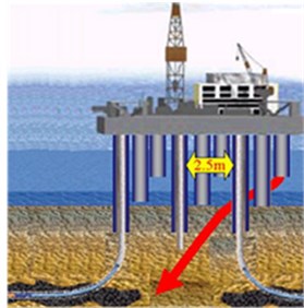
In the marine flatbed, nuclear power stations and oil fields, the marine risers (seen as Fig. 1) and heat exchangers are induced vibrations and even caused failure with cross flow in the fluid filed. To date, most research are numerical simulation and experimental research. Yong-xing lai [1, 2] used computational fluid dynamics software Ansys/Flotran CFD to simulate the flow around circular pipe with fixed, elastic support, and the heat exchanger tube bundle with internal and external fluid.

Fig. 1The marine risers in the ocean

The vortex shedding induced vibration characteristics were calculated for flow around pipe and heat exchanger. Wu Hao [3] used rigid motion equation and newmark integration method to establish a three-dimensional fluid-structure coupling vibration model. The rule of fluid elastic instability was studied for tube bundle with square arrangement. Based on the moving grid method, Ichioka [4] studied fluid elastic vibration for the heat exchanger tube bundle in 1997 and analyzed the vibration regularity of two pipes. Using the finite element method, M. Hassan and M. Hayder [5] simulated fluid elastic vibration of tube bundle with Sagging support in heat exchanger. Y. A. Khulier, S. A. Al-Kaabi, S. A. Said [6] applied node element method and MATLAB finite element program to simulate the fluid elastic vibration of heat exchange tube. F. Oviedo-Tolentino [7] studied the vortex-induced vibration of flexible beam with the bottom of the fixed. Based on the finite volume method and finite element method, Zhi-peng Feng et al. [8-10] used with dynamic grid control technology to analysis the interaction structure and fluid for elastic tubes. In summary, the vortex induced vibration analysis has made great progress for Circular tube and heat exchanger tube bundle. However most of the tube are studied the rigid pipes, and the fluid domain is infinite. Also, the influence of the shape of pipe vibration fluid domain is not considered. In this article, the research of finite fluid elastic instability of flexible pipe was carried out by physical experiment and numerical simulation. The vortex induced vibration characteristics of flexible pipe were analyzed in cylinder fluid field with different positions. It will provide the theory basis for designing and control of the slender flexible pipe such as heat exchanger, marine riser in regarding of vibration.

2. The fluid-structure coupling model of flexible pipe in a cylindrical fluid field with cross flow

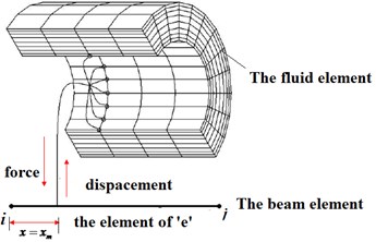
The flexible pipe and the fluid in a cylinder container were selected as research object. The model of fluid-solid coupling model was established for flexible pipe in a limited fluid domain. Seen from Fig. 2, the model was divided into two domains, structural domain $Ω_{s}$ and fluid domain $Ω_{f}$ . The inlet boundary was velocity and it was denoted as $Γ_{D}^{f (1)}$ . The outlet boundary was pressure and it was denoted as $Γ_{N}^{f}$ . The liquid that flowing along the cylinder wall was free sliding surface and it was denoted as $Γ_{D}^{f (2)}$ . In the interaction between fluid and solid, the boundary was fluid-structure coupling and it was denoted as $Γ_{F S I}^{}$ .

The boundary of flexible pipe was hinged on both ends. Assuming that the flexible pipes were uniform and the cross section were circular, if the flexible pipe was dispersed spatial solid element, the model will be too lager and the computational efficiency will be very low. Seen from Fig. 3(a), in this article, the fluid domain was discretized solid elements FLUID142 by computational fluid software CFX. The nodes number was 114345. Seen from Fig. 3(b), the flexible model was adopted Beam188 element by ANSYS software. And the nodes number was 100. And the method of sub regional coupling was adopted to analyze the fluid and solid domain.

Fig. 2The fluid-structure coupling mechanics model of flexible pipe in cylinder fluid domain

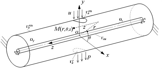
Fig. 3The fluid-structure coupling FEM model of flexible pipe in cylinder fluid domain

a) FLUID142

b) Beam188

3. The fluid-structure coupling numerical calculation method of flexible pipe in a cylindrical fluid field with cross flow

3.1. The control equation of fluid domain

The fluid flowing in cylinder container followed the law of conservation of physical and its continuity equation was shown as:

1

\frac{\partial p}{\partial t} + \frac{\partial (ρ u_{r} r)}{r \partial r} + \frac{\partial (ρ u_{θ})}{r \partial θ} + \frac{\partial (ρ u_{z})}{\partial z} = 0,

where $ρ$ and $p$ are the density and pressure of liquid in the cylinder, respectively. $t$ is time. $u_{r}$ , $u_{θ}$ , $u_{z}$ are the fluid velocity vector along $r$ , $θ$ , $z$ direction, respectively.

The flow regime was turbulent and turbulence model was $k$ - $ε$ . The momentum equation of fluid (navier-stokes equations) was follows:

2

\{\begin{array}{l} \frac{\partial u_{r}}{\partial t} + u_{r} \frac{\partial u_{r}}{\partial r} + \frac{u_{θ}}{r} \frac{\partial u_{r}}{\partial θ} - \frac{u_{θ}^{2}}{r} + u_{z} \frac{\partial u_{r}}{\partial z} = f_{r} - \frac{1}{ρ} \frac{\partial p}{\partial r} + ν_{e f f} (\nabla^{2} u_{r} - \frac{u_{r}}{r^{2}} - \frac{2}{r^{2}} \frac{\partial u_{θ}}{\partial θ}), \\ \frac{\partial u_{θ}}{\partial t} + u_{r} \frac{\partial u_{θ}}{\partial r} + \frac{u_{θ}}{r} \frac{\partial u_{θ}}{\partial θ} - \frac{u_{r} u_{θ}}{r} + u_{z} \frac{\partial u_{θ}}{\partial z} = f_{θ} - \frac{1}{ρ} \frac{1}{r} \frac{\partial p}{\partial θ} + ν_{e f f} (\nabla^{2} u_{θ} - \frac{u_{θ}}{r^{2}} + \frac{2}{r^{2}} \frac{\partial u_{r}}{\partial θ}), \\ \frac{\partial u_{z}}{\partial t} + u_{r} \frac{\partial u_{z}}{\partial r} + \frac{u_{θ}}{r} \frac{\partial u_{z}}{\partial θ} + u_{z} \frac{\partial u_{z}}{\partial z} = f_{z} - \frac{1}{ρ} \frac{\partial p}{\partial z} + ν_{e f f} (\nabla^{2} u_{z}), \end{array}

where $\nabla^{2} = \frac{1}{r} \frac{\partial}{\partial r} (r \frac{\partial}{\partial r}) + \frac{1}{r^{2}} \frac{\partial^{2}}{\partial θ^{2}} + \frac{\partial^{2}}{\partial z^{2}}$ . $f_{r}$ , $f_{θ}$ , $f_{z}$ are volume force along $r,$ $θ,$ $z$ direction, respectively. $ν_{e f f}$ is the effective dynamic viscosity of fluid , $ν_{e f f} = ν + ν_{t}$ . $ν$ , $ν_{t}$ are dynamic viscosity and turbulence viscosity, respectively. It assumed that the turbulent viscosity was connected with turbulent kinetic energy and turbulent kinetic energy dissipation:

3

ν_{t} = C_{μ} ρ \frac{k^{2}}{ε} .

The values of $k$ and $ε$ were solved by turbulent kinetic energy and turbulent kinetic energy dissipation.

The boundary conditions for cylinder fluid domain $Ω_{f}$ were shown as follows:

4

\{\begin{array}{l} u_{r} = n_{f} \cdot u, & o n Γ_{D}^{f (1)}, \\ u_{r} = 0, & o n Γ_{D}^{f (2)}, \\ p_{r} = n_{f} \cdot p_{0}, & o n Γ_{N}^{f}, \end{array}

where $n_{f}$ , $u_{r}$ , $p_{r}$ are unit vector, the velocity vector, stress vector of normal direction at the fluid domain interface, respectively.

The boundary conditions of force and displacement, velocity were seen as section 3.3 at cylinder fluid domain $Ω_{f}$ and solid domain $Ω_{s}$ coupling interface $Γ_{F S I}$ .

3.2. The vibration dynamics equation of flexible pipe

According to the theory of computational structural mechanics, the dynamic equation was obtained for beam element as follows:

5

M {\ddot{d}}_{s} (t) + C {\dot{d}}_{s} (t) + K d_{s} (t) = F (t),

where $M$ , $K$ and $C$ are the mass, stiffness and damping matrix of flexible pipe, respectively. $F (t)$ is the force generated by fluid for flexible pipe in the cylindrical container.

3.3. The force and displacement transfer conditions of flexible pipe in a cylindrical fluid field with cross flow

The force and displacement transfer information were shown in Fig. 4 for the fluid and flexible pipe at the coupled interface. Because of the flexible pipe using beam element and the fluid field using solid element, this led to a serious mismatch at coupling interface. In order to achieve coupling, the condition of displacement, velocity coordination and force balance for structural domain $Ω_{s}$ and fluid domain $Ω_{f}$ at the coupling interface $Γ_{F S I}$ must be all satisfied:

1) Displacement coordination condition:

6

d_{s} \cdot n_{s} + d_{f} \cdot n_{f} = 0,

where $d_{s}$ , $d_{f}$ are the displacement vector of the domain and the fluid domain, respectively.

$n_{s}$ , $n_{f}$ are the unit vector of the domain and the fluid domain, respectively.

Fig. 4The force and displacement interpolation in the coupling interface

2) Velocity coordination condition:

7

{\dot{d}}_{s} \cdot n_{s} + u_{f} \cdot n_{f} = 0,

where ${\dot{d}}_{s}$ , $u_{f}$ are the velocity vector of the domain and the fluid domain, respectively.

3) Force equilibrium condition:

8

σ_{s} \cdot n_{s} + σ_{f} \cdot n_{f} = 0,

where $σ_{s}$ , $σ_{f}$ are the stress vector of the domain and the fluid domain, respectively.

Fig. 5The fluid through the flexible pipe surface in a cylindrical container

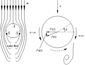
The fluid was flowing in a cylindrical container at a certain speed. And a vortex was forming when flowing around a flexible pipe, which would result in a change in the flow rate. The flow pattern was shown in Fig. 5. The flow pressures $P (θ, z, t)$ which acting on the face, the back and the side surface of the flexible pipe were changed. The $P (θ, z, t)$ belonged to surface load. Integrated with the pressures along the surface of the flexible pipe and two loads which are perpendicular and parallel the fluid flow direction was obtained. The load vertical to the velocity direction was called lift per unit length. And the other load which was parallel to the fluid flow direction was called resistance per unit length. The formulas were shown as follows:

9

\{\begin{array}{l} q_{l}^{e} (z, t) = \int_{0}^{2 π} P (θ, z, t) R s i n θ d θ, \\ q_{d}^{e} (z, t) = \int_{0}^{2 π} p (θ, z, t) R c o s θ d θ, \end{array}

where $σ (P, z, t)$ is fluid pressure of flexible pipe in each point of the cross section at time $t$ . $R$ is the radius of the flexible pipe. And $θ$ was as shown in Fig. 5.

The vector expression of Eq. (9) is:

q^{e} = {[\begin{array}{l} q_{l}^{e} (z, t) & q_{d}^{e} (z, t) \end{array}]}^{Τ} .

As shown in Fig. 2, according to the principle of virtual work, the lift and drag forces that the fluid acting on flexible pipe were equivalent to beam element nodes $i$ and $j$ by coordinate transformation. Thus the nodal forces of the element $e$ on the flexible pipe were obtained as follows:

10

F^{e} = T^{Τ} \int_{0}^{l^{e}} N^{Τ} q^{e} d x,

where $T$ is the coordinate transformation matrix. $N$ is the shape function matrix. $F^{e} = {[\begin{array}{l} F_{l i}^{e} & F_{d i}^{e} & F_{l i}^{e} & F_{l j}^{e} \end{array}]}^{T}$ . They were node lift resistance of flexible pipe beam. Assembling all fluid nodal force on the flexible pipe, the $F (t)$ of Eq. (5) was obtained. Where $F (t) = F_{l} (t) i + F_{d} (t) j$ , $F_{l} (t)$ , $F_{d} (t)$ were the vector of lift force ((the vertical direction of flow)) and drag force (along the direction of flow), respectively. The fluid interface force was applied to flexible pipe beam with equivalent nodal force by interpolation method, which met force equilibrium conditions at coupling interface.

According to the previous document [11] and the assumptions that the cross-section of the pipe was always circular, the nodal displacements of beam element was mapped to the fluid field at the coupling interface. The arbitrary node displacement and velocity vectors in a cartesian coordinate system were expressed as:

11

\{\begin{array}{l} d_{f}^{c} (t) = H_{Γ_{F S I}}^{Τ} (t) d_{s} (t), \\ u_{f}^{c} (t) = H_{Γ_{F S I}}^{Τ} (t) {\dot{d}}_{s} (t), \end{array}

where: $d_{f}^{c} (t)$ , $u_{f}^{c} (t)$ were the displacement and velocity vector at coupling interface in fluid domain.

$H_{Γ_{F S I}}^{Τ} (t)$ was grid interpolation function matrix at fluid-structure coupling interface.

According to the transform relationship between cylindrical coordinate system and cartesian coordinate system, the displacements $d_{f}^{c} (t)$ and velocity $u_{f}^{c} (t)$ in the Eq. (11) were converted to $d_{f}^{} (t)$ and $u_{f}^{} (t)$ in cylindrical coordinates. Thus it achieved displacement harmonization for structural domain and fluid domain at coupling interface.

3.4. The algorithm for flexible pipe in a cylindrical fluid field with cross flow

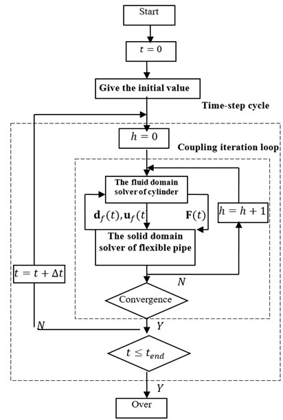
The coupling iteration block diagram was shown in Fig. 6 for flexible pipe in a cylindrical fluid field with cross flow. $t$ was the current time step. $h$ was the coupling iteration number in current time step.

(1) Give inlet velocity $u$ and outlet pressure $P$ .

(2) Solve the fluid domain $Ω_{f}$ and get the coupling interface load $P (θ, z, t)$ ;

(3) Transfer the physical of fluid domain interface to structural domain interface, get the coupling interface loads $F (t)$ of domain interface;

(4) Solve structural domain $Ω_{s}$ , get displacement $d_{s} (t)$ and velocity ${\dot{d}}_{s} (t)$ at coupled interface in structural domain.

(5) Transfer the physical of structural domain interface to fluid domain interface, get displacement $d_{f} (t)$ and velocity $u_{f} (t)$ at coupled interface in fluid domain.

(6) Order $t = t + Δ t$ , follow the previous coupling step iteration (2) to (5), and do the current time step of coupled iterative calculation.

Fig. 6The geometric location of the flexible pipe in the cylindrical container

4. The analysis study of vibration characteristics for flexible pipe in cylindrical fluid

4.1. Cases and calculation parameters

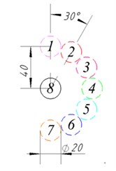
The calculation parameters of the flexible pipe and fluid were listed in Table 1.

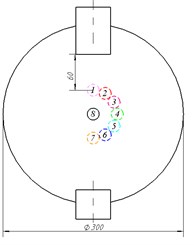
The flexible pipe was placed in a cylindrical container with the position 1 to 8. And the geometric position was as shown in Fig. 7. The flexible pipe at different positions was calculated by the model and calculation methods established in this paper. Then, the lift and drag curves, and induced vibration regularity of flexible pipe were obtained as followed.

Table 1The calculation parameters of the flexible pipe and fluid

Length (m)	1.8
Outer diameter (m)	0.02
Inner diameter (m)	0.016
Elastic modulus (GPa)	2.9
Poison’s ratio	0.3
The density of flexible pipe (kg/m³)	1140
The density of fluid (kg/m³)	1000
Dynamic viscosity (mPa^.s)	1
Inlet velocity (m/s)	2.236
outlet pressure (MPa)	0
Natural frequency of pipe (Hz)	23.91
Calculation time step (s)	0.001

Fig. 7The geometric location of the flexible pipe in the cylindrical container

4.2. The pressure analysis of flexible pipe in fluid region

4.2.1. The fluid velocity and pressure of flexible pipe’s cross section at center position

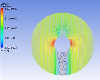
The Fig. 8 was the streamlines for flexible pipe placed in the cylindrical container position 1 when $t =$ 1.8 s. The Fig. 9 was the velocity distribution on the cross section for flexible pipe in different positions. Seen from Figs. 8, 9, the velocity was uniform on the cross-section of the flexible pipe in different positions. The value of velocity was small at the upstream face ( $θ =$ 90°). The value of velocity was large at lateral face (90° $< θ <$ 225^o, 315° $< θ <$ 360°(0°), 0° $< θ <$ 90°). The value was almost zero at lee face (225° $< θ <$ 315°).

Fig. 8The streamlines for flexible pipe placed in the cylindrical container position 1 when t= 1.8 s

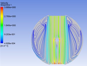
a) The entire

b) The local

The Fig. 10 was the turbulent vortex for flexible pipe placed in the cylindrical container position 1 when $t =$ 1.8 s. Seen from Fig. 10, there was almost no turbulent vortex at upstream face. In the side stream surface, the turbulent vortex was produced gradually. When $θ =$ 225° and $θ =$ 315°, its vortex momentum was maximized.

Fig. 9The velocity distribution on the cross section for flexible pipe in different positions

a) 1, 7, 8

b) 4, 8

Fig. 10The vortex shedding for flexible pipe placed in the cylindrical container position 1 when t= 1.8 s

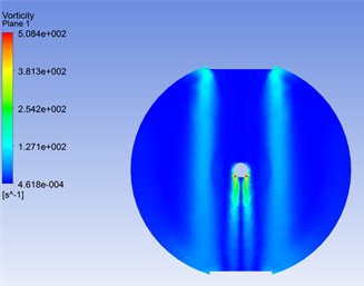
a) The entire

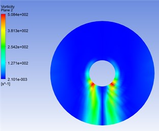
b) The local

Fig. 11The stress distribution on the cross section for flexible pipe in different positions

a) Perpendicular to the flow direction

b) Along the flow direction

The pressure distribution of the flexible pipe in different locations was shown in figure 11. Of note, the fluid pressure on flexible pipe’s cross-section was changed with positions. In 48°-132°, namely in the position of upstream face, the fluid pressure was positive, greater than atmospheric pressure and the maximum value was changed with positions. In the position of 1, 7, 8 (facing the inlet flow rate), the maximum fluid pressure was occurred in the surface facing the flow at 90°. In 48°-132°, namely in the position of lee face, the fluid pressures were relatively positive, greater than atmospheric pressure. the maximum pressure was occurred at 234°-240°. But the change of maximum value was very small with varying positions of the flexible pipe.

In 132°-210°, 330°-360°, 0°-48°, namely in the position of side face, the fluid pressures were relatively negative, less than atmospheric pressure and the maximum negative value was occurred in 174° and 6° position.

To sum up, the fluid pressure in the upstream face was greater than the value in the lee face. The pressure in the lee face was greater than the value of side flow face.

4.2.2. Lift and drag force

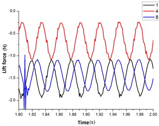
The Fig. 12 was the lift force curves for the flexible pipe at the position 1, 4, 8. From the Fig. 12(a), it showed that the initial lift force was great for flexible pipe at the position 8 (deviating the entrance). The value decayed rapidly from time 0 s to 0.5 s. While the value was small at the position of 1, 8 (facing the entrance). In $t >$ 0.5 s, the value of lift force was stabilized. From the Fig. 12(b), when the vibration of the flexible pipe was stable, the life force curve was sine or cosine. The amplitude of sine or cosine curve was symmetrical at the position 1,8 and the upper and lower vibration value was from –0.34 N to 0.34 N. While the amplitude of sine or cosine curve was asymmetric at the position 4 and the upper and lower vibration value was from –0.5 N to 0.74 N. The magnitude at position 4 was significantly greater than the value at the position 1, 8.

Fig. 12The lift force curves of changing with time for flexible pipe placed in the cylindrical container position 1, 4, 8

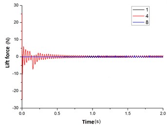
a) 0.0 s-2.0 s

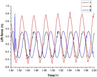
b) 1.8-2.0 s

Fig. 13The resistance curves of changing with time for flexible pipe placed in the cylindrical container position 1, 4, 8

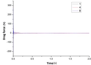
a) 0.0 s-2.0 s

b) 1.8-2.0 s

The Fig. 13 was the drag force curves of flexible pipe at the position 1, 4, 8. From the Fig. 13(a), the initial value was large. From $t =$ 0 s to $t =$ 0.3 s, the value decreased rapidly. At $t >$ 0.3 s, the value was stabilized. From the Fig. 13(b), the drag curve was also sine or cosine and the drag’s magnitude at position 4 was significantly greater than the value at the position 1, 8.

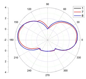
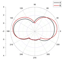
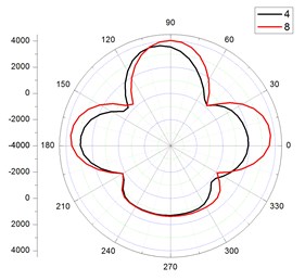
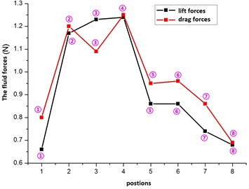
The Fig. 14 showed that, when the flexible pipe at the position 2, 3, 4, the lift and drag forces’ amplitude was large. While at the position 5, 6, 7, 8, the amplitude was small.

Fig. 14The fluid forces for flexible pipe placed in the cylindrical with different positions

4.3. The vortex induced vibration analysis of flexible pipe

4.3.1. Acceleration

The Fig. 15 was the acceleration curves of the flexible pipe at position 1, 4, 8 in a direction perpendicular to the flow rate. From the Fig. 11(a), when the flexible pipe located at position 1, 8 (facing the entrance), its acceleration value was small at $t =$ 0 s-0.5 s. At $t =$ 0.5 s-0.75 s, the acceleration’s amplitude increased quickly. At $t >$ 0.75 s, the amplitude vibration was stabilized.

From the Fig. 15(b), when the vibration was stable, the acceleration curve that was perpendicular to the direction of flow was a sine or cosine curve. And the acceleration amplitude at position 4 was significantly greater than the value at the position 1, 8.

Fig. 15The acceleration curves of changing with time for flexible pipe placed in the cylindrical container position 1, 4, 8

a) 0.0 s-2.0 s

b) 1.8-2.0 s

Fig. 16The acceleration curves of changing with time for flexible pipe placed in the cylindrical container position 1, 4, 8

a) 0.0 s-2.0 s

b) 1.8-2.0 s

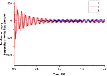
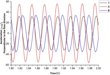
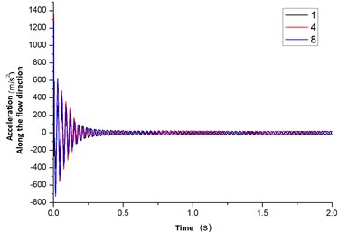
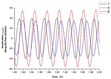
The Fig. 16 was the acceleration curves of flexible pipe at position 1, 4, 8 in a direction along the flow rate. The Fig. 16(a) showed that the fluid begun to flow into the container, which leads to a larger acceleration along the flow rate’s direction. In $t =$ 0-0.4 s, the acceleration decayed quickly. In $t >$ 0.8 s, the acceleration was stabilized. From the figure 16 (b), the acceleration curve which was along the direction of flow was a sine or cosine curve. And the acceleration amplitude at position 4 was significantly greater than the value at the position 1, 8 too.

Fig. 17The maximum value of acceleration and velocity for flexible pipe placed in the cylindrical with different positions

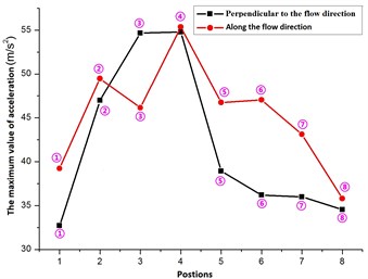
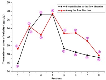
The Fig. 17 showed that, when the flexible pipe located at different positions, since the fluid elastic instability affected, it resulted in different amplitudes of acceleration and velocity. When the flexible pipe located at position 3, the acceleration, velocity that was vertical to the flow velocity direction was greater than the value along the flow velocity direction. Therefore, the main vibration direction was the direction that was perpendicular to the flow rate for flexible pipe at the position 3.

At position 4, the acceleration and velocity were identical along two directions. Namely, the vibration of flexible pipe was same along two directions.

When the flexible pipe located at position 1, 2, 5, 6, 7, 8, the acceleration, velocity that was vertical to the flow velocity direction was less than the value along the flow velocity direction. And therefore the main vibration direction was the direction that was along the flow rate for flexible pipe at the position 1, 2, 5, 6, 7, 8.

It can be seen from the Fig. 17, when the flexible pipe located at position 4 (deviation from the inlet velocity), the vibrations along two directions were larger than the other positions and the maximum accelerations that are vertical and parallel to the flow velocity direction are 54.79 m/s², 55.36 m/s², respectively. While at position 1, 7, 8 (facing the inlet velocity), the vibrations along two directions were less than the other positions and the maximum accelerations that were vertical and parallel to the flow velocity direction were respectively 34.54 m/s², 35.8 m/s² at the position 8.

4.3.2. Movement track and ultimate annulus

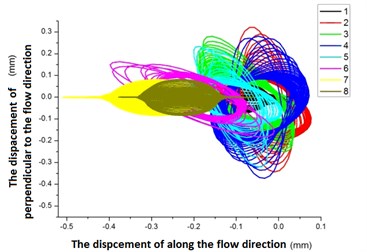
The displacements of flexible pipe were set as $X$ -coordinate, $Y$ -coordinate respectively. The movement track was obtained for flexible pipe at different positions and seen as Fig. 18.

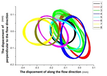
The Fig. 18(a) showed that, when the fluid begun to flow into the cylindrical container, the flexible pipe started vibrating in the effect of fluid and its movement track was “shuttle” shape. The Fig. 18(b) showed that, with the fluid flowing into the cylindrical container, the vibration of flexible pipe was stable and its trajectory was “oval”.

When the flexible pipe was situated at 1, 7, 8 position, the size of the ellipse was less and the vibration level was similar at the position 1, 7, 8.

When the flexible pipe was situated 2, 3, 4, 5, 6, position, the trajectory of the flexible tube was still ellipse, but the ellipse rotated a certain angle with respect to the oval of position 8.

The Fig. 19 is the limit cycle and cycle for flexible pipe placed in the cylindrical with different positions. From the Fig. 15, the acceleration in the vertical direction of flow is a sine or cosine curve for flexible pipe. Then the displacement and velocity curves are also sine or cosine. Assuming that displacement equation in the direction of vertical velocity was: $x = A c o s (ω t + φ)$ , Where in it, $A$ was the amplitude, $ω$ was angular frequency and $φ$ was the phase angle at the direction of the vertical velocity. The velocity equation of flexible pipe was: $v_{x} = \dot{x} = - A ω s i n (ω t + φ)$ . Elimination parameters, the displacement and velocity equation was:

{(\frac{x}{A})}^{2} + {(\frac{\dot{x}}{A ω})}^{2} = 1 .

The graphs enclosed by displacement and velocity were ellipse, known as “Limit Cycles”. Seen from the Fig. 18(a), the long axis of ellipse was the amplitude A. The minor axis was $A ω$ .

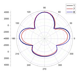
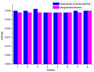
Fig. 19(a) shows that the proportion of minor axis and long axis is approximately equal at different positions, which is $A ω / A = ω .$ Namely the vibration frequency and cycle are tantamount. The Fig. 19(b) shows that the cycles are 0029 s-0.03 s for flexible pipe in different positions.

Fig. 18The trajectory for flexible pipe placed in the cylindrical with different positions

a) Before stable

b) After stable

Fig. 19The limit cycle and cycle for flexible pipe placed in the cylindrical with different positions

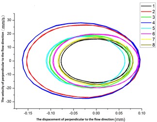
a) Limit cycle

b) Cycle

4.4. The contrast of numerical simulation and text

4.4.1. The experimental apparatus and principle

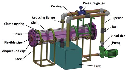
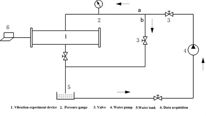
As shown in Fig. 20, according to geometric similarity and kinematic similarity, vibration test was designed for flexible pipe in cylindrical fluid domain. Its circulatory system was shown in Fig. 21. The water was delivered into the pipe from the tank 5 by pump 4. Through the valve 3, the water was flowing into inlet $a$ and $b$ . The water flowing into inlet a was entering the induced vibration test equipment 1. The valve 3 was used to adjust the fluid velocity.

In the test, the length of pipe was 1.8 m and the medium was water. The inlet flow rate was 2.236 m/s. The experiment was carried out for flexible pipe at 8 positions (seen from Fig. 7). Using GWT-2B-axis accelerometer to monitor the vibration, the acceleration curve was acquired for flexible pipe.

Fig. 20The vibration test device for flexible pipe in a cylindrical fluid domain

a) The schematic diagram

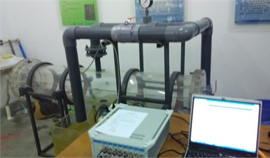
b) The experimental device

Fig. 21The vibration test circulatory system for flexible pipe in a cylindrical fluid domain: 1 – vibration experiment device, 2 – pressure gange, 3 – valve, 4 – water pump, 5 – water tank, 6 – data acquisition

The vibration test circulatory system for flexible pipe in a cylindrical fluid domain: 1 – vibration experiment device, 2 – pressure gange, 3 – valve, 4 – water pump, 5 – water tank, 6 – data acquisition

4.4.2. The comparison results

The Fig. 22 was the vibration acceleration curve for flexible pipe at the location 8. It showed that the experimental acceleration value was upper and lower, while numerical simulation acceleration value was cyclical variation. The average acceleration amplitude was seen in Table 2 for the flexible pipe at the location of 1 to 8.

Fig. 22The acceleration curves of changing over time for flexible pipe with the position of 8 in the cylindrical fluid domain

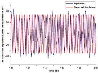
a) Perpendicular to the flow direction

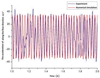
b) Along the flow direction

From Table 2, there were 32 groups of acceleration value from experimental measurement and numerical simulation at the position from 1 to 8. There were 8 groups with errors were greater than 10 % and the remaining were less than 10 %. That was the acceleration value of numerical simulation was agreement with the value of experimentally measured. Therefore, it proved that the theoretical model and calculation method established in this paper correct.

Table 2The compared results between experimental and numerical simulation for flexible pipe in different positions

Positions			1	2	3	4	5	6	7	8
The acceleration of perpendicular to the flow direction (m/s²)	Max	Experiment	30.54	56.32	35.32	40.21	37.55	32.12	37.55	32.12
		Numerical simulation	32.70	46.98	38.93	36.19	35.99	34.54	35.99	34.54
		Error	7.07	–16.58	10.22	–10.00	–4.15	7.53	–4.15	7.53
	Min	Experiment	–30.93	–56.98	–34.78	–39.58	–37.58	–35.02	–37.58	–35.02
		Numerical simulation	–32.89	–47.80	–38.57	–37.06	–36.38	–36.4	–36.38	–36.4
		Error	6.34	–16.11	10.90	–6.37	–3.19	3.94	–3.19	3.94
The acceleration of along the flow direction (m/s²)	Max	Experiment	42.10	40.20	49.23	47.35	41.09	35.75	41.09	35.75
		Numerical simulation	39.23	49.48	46.75	47.05	43.13	35.8	43.13	35.8
		Error	–6.82	23.08	–5.04	–0.63	4.96	0.14	4.96	0.14
	Min	Experiment	–40.18	–45.98	–48.33	–45.12	–40.02	–34.89	–40.02	–34.89
		Numerical simulation	–39.51	–50.43	–46.95	–46.80	–43.28	–35.10	–43.28	–35.10
		Error	–1.67	9.68	–2.86	3.72	8.15	0.60	8.15	0.60

5. Conclusions

1) With selected flexible pipe and fluid in a cylinder container, the model of fluid-solid coupling model was established for flexible pipe in a limited fluid domain. The flexible pipe was dispersed into several three-dimensional beam element and the fluid domain is discretized into solid element. And the method of sub regional coupling was adopted to analyze the fluid and solid domain.

2) According to the geometric similarity and kinematic similarity, the vibration test equipment was designed for flexible pipe in cylindrical fluid domain. Using GWT-2B-axis accelerometer to monitor the vibration, the results were compared to the numerical simulation and the degree of agreement was reached 75 %.

3) The vibration characteristics were studied for the flexible pipe in cylindrical fluid domain at different positions. The results indicated that when the flexible pipe in position 4 (departing from the inlet velocity position), the acceleration values were greater than that of other positions. While in the position of 1, 7, 8 (facing on the inlet velocity position), the acceleration and velocity values were less than at other locations.

To sum up, to reduce the vortex-induced vibration, the flexible pipe should be placed in facing to the direction of the inlet flow rate. The greater the deviation from the inlet velocity position, the stronger the vibration is. We should try to avoid placing the flexible pipe in a position deviated from the inlet flow rate.

References

Lai Yongxing, Liu Minshan, Dong Qiwu Numerical simulation of induced vibration for viscous flow past a circular cylinder. Journal of Dynamics and Control, Vol. 3, Issue 1, 2005, p. 86-91.

Search CrossRef
Lai Yongxing, Liu Minshan, Dong Qiwu Dynamic characteristic analysis of heat exchanger tube bundles with internal and external fluid. Journal of Vibration and Shock, Vol. 25, Issue 2, 2006, p. 159-162.

Search CrossRef
Wu Hao, Tan Wei, Nie Qing-de A numerical model for fluid-elastic instability of a square tube array. Journal of Vibration and Shock, Vol. 32, Issue 21, 2013, p. 102-106.

Search CrossRef
Ichioka T., Kawata Y., Nakamura T., et al. Research on fluid elastic vibration of cylinder arrays by computational fluid dynamics: analysis of two cylinder and a cylinder row. JSME International Journal Series B, Fluids and Thermal Engineering, Vol. 40, Issue 1, 1997, p. 16-24.

Publisher
Hassan M., Hayder M. Modelling of fluid elastic vibrations of heat exchanger tubes with loose supports. Nuclear Engineering and Design, Vol. 238, 2008, p. 2507-2520.

Publisher
Khulief Y. A., Al-Kaabi S. A., Said S. A. Prediction of flow-induced vibrations in tubular heat exchangers – Part 1: numerical modeling. Journal of Pressure Vessel Technology, Vol. 131, 2009, p. 011301-011308.

Publisher
Oviedo-Tolentino F., Pérez-Gutiérrez F. G., Romero-Méndez R. Vortex-induced vibration of a bottom fixed flexible circular beam. Ocean Engineering, Vol. 88, 2014, p. 463-471.

Publisher
Feng Zhi-peng, Zhang Yi-xiong, Zang Feng-gang Analysis of vortex-induced vibration characteristics for a three dimensional flexible tube. Applied Mathematics and Mechanics, Vol. 34, Issue 9, 2013, p. 976-985.

Search CrossRef
Feng Zhi-peng, Zang Feng-gang, Zhang Yi-xiong Theoretical model and numerical simulation of vortex induced flexible tube vibration. Applied Mathematics and Mechanics, Vol. 35, Issue 5, 2014, p. 581-588.

Search CrossRef
Feng Zhi-peng, Zhang Yi-xiong, Zang Feng-gang Numerical simulation of fluid-structure interaction for tube bundles. Applied Mathematics and Mechanics, Vol. 34, Issue 11, 2013, p. 1165-1172.

Search CrossRef
Liu Ju-bao, Luo Min, Wang Lin Methodology of fluid-structure interaction of rotary slender beam in pipe. Engineering Mechanics, Vol. 28, Issue 4, 2011, p. 251-256.

Search CrossRef

About this article

Received

09 October 2015

Accepted

18 January 2016

Published

30 June 2016

SUBJECTS

Flow induced structural vibrations

DOI

https://doi.org/10.21595/jve.2016.16547

Keywords

vortex-induced vibration

flexible pipe

fluid-structure

at different positions

Acknowledgements

This work was supported by the Project of National Natural Science Fund (11272085) and the China National Petroleum Corporation Scientific Research and Technology Development Projects (2013E-3807-01).

This is an open access article distributed under the Creative Commons Attribution License, which permits unrestricted use, distribution, and reproduction in any medium, provided the original work is properly cited.

Previous article in issue Previous Next article in issue Next

Research article

2022 06 13

Numerical simulations on VIV of a flexible cylinder under two degree-of-freedoms excitations

Di Deng, Weicai Peng

Research article

2020 05 15

Effects of variable parameters on the behaviour of the single flexibly-mounted rod in a closely-packed array

Sabine Upnere, Normunds Jekabsons, Sergejs Dementjevs, Michael Wohlmuther

Research article

2019 11 28

Numerical simulation of vortex induced vibrations on a circular cylinder at different Reynold’s number

Shivam Yadav, Akshaj Kulshreshtha, Baij Nath Singh

Research article

2018 02 15

Wake and structure model for simulation of cross-flow/in-line vortex induced vibration of marine risers

Younes Komachi, Said Mazaheri, Mohammad R. Tabeshpour

J.-B. Liu, Q.-B. Yue, R.-Z. Dong, and Q. Zhang, “The analysis of vortex induced vibration of the flexible pipe in a cylindrical fluid field with cross flow,” Journal of Vibroengineering, Vol. 18, No. 4, pp. 2403–2417, Jun. 2016, https://doi.org/10.21595/jve.2016.16547

Copy Extrica

Copied to clipboard!

TY  - JOUR
DO  - 10.21595/jve.2016.16547
UR  - https://doi.org/10.21595/jve.2016.16547
TI  - The analysis of vortex induced vibration of the flexible pipe in a cylindrical fluid field with cross flow
T2  - Journal of Vibroengineering
AU  - Yue, Qian-Bei
AU  - Liu, Ju-Bao
AU  - Dong, Ri-Zhi
AU  - Zhang, Qiang
PY  - 2016
DA  - 2016/06/30
PB  - JVE International Ltd.
SP  - 2403-2417
IS  - 4
VL  - 18
SN  - 1392-8716
ER  - 

Copy Ris

Copied to clipboard!

@article{Yue_2016,
	doi = {10.21595/jve.2016.16547},
	url = {https://doi.org/10.21595/jve.2016.16547},
	year = 2016,
	month = {jun},
	publisher = {{JVE} International Ltd.},
	volume = {18},
	number = {4},
	pages = {2403--2417},
	author = {Qian-Bei Yue and Ju-Bao Liu and Ri-Zhi Dong and Qiang Zhang},
	title = {The analysis of vortex induced vibration of the flexible pipe in a cylindrical fluid field with cross flow},
	journal = {Journal of Vibroengineering}
}

Copy Bibtex

Copied to clipboard!

[1]Q.-B. Yue, J.-B. Liu, R.-Z. Dong, and Q. Zhang, “The analysis of vortex induced vibration of the flexible pipe in a cylindrical fluid field with cross flow,” Journal of Vibroengineering, vol. 18, no. 4, pp. 2403–2417, Jun. 2016, doi: 10.21595/jve.2016.16547.

Copy IEEE

Copied to clipboard!

Yue, Qian-Bei, Ju-Bao Liu, Ri-Zhi Dong, and Qiang Zhang. “The Analysis of Vortex Induced Vibration of the Flexible Pipe in a Cylindrical Fluid Field with Cross Flow.” Journal of Vibroengineering 18, no. 4 (June 30, 2016): 2403–17. https://doi.org/10.21595/jve.2016.16547.

Copy Chicago

Copied to clipboard!

The analysis of vortex induced vibration of the flexible pipe in a cylindrical fluid field with cross flow

Abstract

1. Introduction

2. The fluid-structure coupling model of flexible pipe in a cylindrical fluid field with cross flow

3. The fluid-structure coupling numerical calculation method of flexible pipe in a cylindrical fluid field with cross flow

3.1. The control equation of fluid domain

3.2. The vibration dynamics equation of flexible pipe

3.3. The force and displacement transfer conditions of flexible pipe in a cylindrical fluid field with cross flow

3.4. The algorithm for flexible pipe in a cylindrical fluid field with cross flow

4. The analysis study of vibration characteristics for flexible pipe in cylindrical fluid

4.1. Cases and calculation parameters

4.2. The pressure analysis of flexible pipe in fluid region

4.2.1. The fluid velocity and pressure of flexible pipe’s cross section at center position

4.2.2. Lift and drag force

4.3. The vortex induced vibration analysis of flexible pipe

4.3.1. Acceleration

4.3.2. Movement track and ultimate annulus

4.4. The contrast of numerical simulation and text

4.4.1. The experimental apparatus and principle

4.4.2. The comparison results

5. Conclusions

References

About this article

Related Articles