Abstract
In this paper, active control with time delay was implemented for eliminating the vibration of the non-linear system excited by external and parametric forcing amplitude in the presence of 1:4 internal resonances. Multiple time scale method is applied to determine first-order approximations of the controlled system. The stability of the system is investigated analytically using Lyapunov first method and numerically using frequency, force-response curves and phase-plane method for the considered resonance case. Effects of different parameters on the steady state response of the controlled system are investigated. Variation of some parameters leads to the bending of the frequency, force-response curves and hence to the jump phenomenon occurrence.
1. Introduction
The dynamics models of many engineering applications involve nonlinearities, time delay and uncertain parameters and are they are naturally described by nonlinear differential difference equation systems. Time delays often occur due to dead time associated with measurement sensors, transportation lag such as in flow through pipes, and approximation of higher order dynamics. On the other hand, uncertainty can cause modelling errors, parametric variations and external disturbance. The presence of time-delays and uncertain parameters, if it is nor appropriately accounted for in the design of the controller, may produce unacceptable limitations on the achievable control quality and may cause serious problems. Control theory is an interdisciplinary branch of applied mathematics. Since its introduction in 1980’s, it has grown to become an interest scientific domain. The problem of stability of nonlinear time-delay systems has been investigated intensively during the past decades [1-3]. Here there are two principal approaches, the first one is based on the Razumikhin theorem, and the other one is based on the Lyapunov-Krasovskii functionals. These two approaches were successfully applied by different authors to the study of wide classes of dynamical systems [1-5]. Stability may depend on delay, and in this case, when delay exceeds a certain value, we cannot guarantee that the dynamical system remains in stable region. In some engineering applications, the smallness of delay cannot be assured. Moreover, the delay value may be unknown. Therefore, it is important to study stability conditions under which the dynamical system remains stable for any positive value of delay.
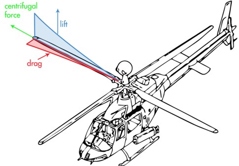
Vibrations and dynamic chaos are undesired phenomenon in structures as they cause the 4D. They are: disturbance, discomfort, damage and destruction of the system or the structure. For these reasons, money, time and effort are spent to eliminate or control vibrations, noise and chaos or to minimize them. Structures and mechanical systems should be designed to enable better performance under different types of loading, particularly dynamic and transient loads. Mechanical resonance is the tendency of a mechanical system to respond at greater amplitude when the frequency of its oscillations matches the system’s natural frequency of vibration (its resonance frequency or resonant frequency ) than it does at other frequencies. It may cause violent swaying motions and even catastrophic failure in improperly constructed structures including bridges, buildings and airplanes-a phenomenon known as resonance disaster. Vibration control is classified into two main categories: passive control and active control. In many engineering applications, active controller (control signal and feedback signal with natural frequency ) was added. In Helicopters blade, we need to add a controller to reduce the shaft torque, and to improve rotor performance.
Unfortunately, active control techniques may suffer from a time delay caused by transport delay, measurements of the system states, online computation, filtering and processing of data and executing of control forces as required in control processing. The stability issue and the delayed control systems performance are of theoretical and practical importance. Therefore, the studies of control system with time delay have been developed by many researches in last two decades. Time-delays phenomena, which are especially prevalent if a control system is being implemented in mechanical or structural systems, can limit the performance of the feedback controllers. In many systems, unavoidable time-delays in controllers give rise to complicated system behavior and can cause instability of the dynamic systems. On the other hand, time-delays can deliberately be used to achieve better dynamical system behavior when control is applied with the time delays. Many passive and active control techniques are used to eliminate (suppress) the vibration to a minimum level. Yabuno and Jo [6] studied the effects of parametric resonance due to the asymmetric non-linearity of a restoring force. Jo and Yabuno [7, 8] worked on the amplitude reduction of the primary and parametric resonance of a nonlinear oscillator using a passive controller. Amer et al. [9] discussed two active control laws based on linear negative velocity and acceleration feedback. Nonlinear string-beam coupled systems subjected to mixed forces are studied by Hamed et al. [10]. Sayed and kamel [11, 12] applied different controllers on the vibrating system to eliminate the vibration of the rotor blade flapping motion. The effects of different terms (quadratic and cubic) on nonlinear dynamic characteristics under mixed excitations are investigated by Sayed and Mousa [13]. An analytical analysis of the nonlinear dynamics of a symmetric cross-ply composite laminated piezoelectric plate under mixed excitations is investigated by Sayed and Mousa [14]. They verified the analytical results by multiple time scale method with the numerical results of the modal equations. Sayed and Hamed [15], studied the stability of the nonlinear rotor-seal system using Liapunov’s first method. The effects of various parameters on the behavior of the system and stability of the system are investigated numerically by response curve. Poincaré maps are used to determine stability and plot bifurcation diagrams. Warminski et al. [16] investigated active suppression of non-linear composite beam vibrations by using selected control algorithms. Shin et al. [17] investigated active control of clamped beams using PPF (Positive Position Feedback) controllers. Eissa and Sayed [18-20], investigate the influences of different controllers (negative velocity feedback, its square and its cubic) on simple pendulum and spring pendulum in the case of primary resonance. Das and Chatterjee [21] studied delay differential equations (DDEs) close to Hopf bifurcations. Ahlborn and Parlitz [22] discussed different delay feedback control with different and independent delay times to stabilize steady states of various chaotic dynamical systems. Gjurchinovski et al. [23] studied the stabilization of unstable steady states by delayed feedback control in the regime of a high-frequency. Zhao and Xu [24] investigated the effects of delayed feedback suppress the vibration of vertical displacement in a two-degrees-of-freedom nonlinear dynamic system to external excitations. Zhao and Xu [25] investigated the delayed feedback control and saturation control to eliminate the vibration of a dynamical system. Xu et al. [26] studied the effect of time delays on the saturation control of the first-mode vibration in stainless-steel beam. Maccari [27] investigated vibration control for the primary resonance of a cantilever-beam. Jnifene [28] studied active control of flexible structures by applying delayed position feedback. Chatterjee [29] make a study to time-delay feedback control for controlling friction-induced instability. Saeed et al. [30] proposed controller for active suppression of nonlinear beam vibrations based on time delay saturation, also they investigate the effects of time-delay on dynamical system behaviour. Song and He [31] studied finite-time passive control for a class of nonlinear systems with time-delays and under uncertainties. Elnaggar and Khalil [32] have presented an analysis of primary, superharmonic of order five, and subharmonic of order one-three resonances for non-linear non-linear single-degree-of-freedom system with two distinct time-delays under an external excitation.
In [12] the authors study two different controllers 1:2 ) and 1:3 () without time-delay. In this paper we investigated another different controller 1:4 ) with time-delay for reducing the vibration of the non-linear dynamical system excited by external and parametric forcing amplitude. Moreover, stability analysis was studied in order to declare the optimal range of the parameters to avoid resonance disaster. This paper is organized as follows. Section 2 describes the equation of motion of helicopter rotor blade flapping. Section 3 introduces the multiple time scales method to solve the system of equations. Section 4 describes the stability of the system and their results. Section 5 the numerical results are presented. Finally, Section 6 presents our conclusions.
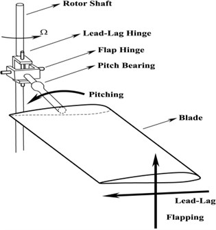
Fig. 1Model of helicopter rotor blade flapping motion
2. Equations of motion
The governing equations of a non-linear system with quadratic and cubic nonlinearities excited by mixed forcing amplitudes which describing the vibration of helicopter rotor blade flapping motion (shown in Fig. 1) under active control are in the following form:
where, and denotes the response of the plant and controller, , are the damping ratio of the plant and controller, , are control signal and feedback signal respectively, and , are the curvature non-linear coefficients. Also, the natural frequency of the main system (plant), the natural frequency of the controller, , are the forcing frequencies, and are the external and parametric forcing amplitudes and 1 is a small perturbation parameter.
We choose the control signal and the feedback signal , where and are positive constant gain, , , , are the time delays. We applied the method of multiple time scale to obtain the response of the given system near the simultaneous resonance , in the presence of 1:4 internal resonance . The stability of the system is investigated analytically using Lyapunov first method and numerically using frequency, force-response curves and phase-plane method for the considered resonance case.
3. Mathematical analysis
We use multiple time scales method [33-35] to obtain a first order approximation of Eqs. (1) and (2) in the form:
where is a fast time scale associated with changes occurring at the frequencies , and , and is a slow time scale characterizing the modulation in the amplitudes and phases of the motion. In terms of and , the time derivatives are transformed into:
where and . Substituting Eqs. (3)-(4) into Eqs. (1)-(2), and equating the coefficients of the same order of in both sides, we obtain the following:
Order
Order
The general solutions of Eqs. (5) and (6), can be written in the form:
where refers for the complex conjugate of the preceding terms. The quantities and are unknown at this stage of the analysis. They will be determined by eliminating the secular and small-divisor terms at the next approximation. Substituting Eqs. (9) and (10) into Eqs. (7) and (8), the following are obtained:
The closeness of the resonances in the case of simultaneous primary and principal parametric resonance (where , ), in the presence of 1:4 internal resonance can be described quantitatively by introducing the detuning parameters , and according to:
Substituting Eq. (13) into Eqs. (11)-(12) and eliminating the secular terms, we obtain the solvability conditions:
We express the functions and in the polar form as:
where , , and are functions of . Putting Eq. (16) into Eqs. (14) and (15) and separating the real and imaginary parts, we get:
Then, it follows from Eq. (21) that:
Substituting Eq. (22) into Eqs. (18) and (20), we obtain:
From Eqs. (17), (19), (23) and (24), the autonomous system equations are:
4. Equilibrium solution
At the steady state motions we have:
Then it follows from Eq. (22) that:
Hence, the steady state solutions of Eqs. (25)-(28) are given by:
4.1. Stability analysis
To derive the stability criteria, we need to examine the behavior of small deviations from the steady state solutions and . Thus, we assume that:
where and are the solutions of Eqs. (31)-(34) and , are perturbations which are assumed to be small compared with and . Substituting Eq. (35) into Eqs. (25)-(28), using Eqs. (31)-(34) and keeping only the linear terms in , we obtain:
The stability of the system is determined by examining the eigenvalues of the Jacobian matrix of the right-hand sides of Eqs. (36)-(39). If the real part of each eigenvalues of the Jacobian matrix is negative, the corresponding equilibrium solution is asymptotically stable. If the real part of any of the eigenvalues is positive, the corresponding equilibrium solution is unstable.
5. Numerical results
Results are obtained in graphical forms as steady state amplitudes versus time-delay , , , , forcing amplitudes , and detuning parameter and as time history or the response for both main system and controller 1:4 internal resonance. The various parameters of the main system and controller in Figs. 2-9 are 0.01, 0.001, 0.03, 0.015, 0.8, 2, , 0.2, 0.4. Solid lines denote to stable solutions on the response curves, while dotted lines denote to unstable solutions and asterisks are the boundary between stable and unstable solutions.
5.1. Effects of time-delays
Fig. 2 shows the response curves of amplitude-delay for . From this figure, we noticed that time delay should be chosen in the intervals [0, 0.252] and [2.885, 3.395]. Away from these ranges the saturation controlled system losses stabilities. Fig. 3 shows the response curves of amplitude-delay for . It can observe that the response curves are stable in the delay intervals [0, 0.514] and [5.777, 6.797]. For other range of the saturation controlled system becomes unstable. Fig. 4 shows response curves of amplitude-delay for The amplitude response curves have two stable ranges [0, 1.028] and [11.553, 13.594]. The saturation controlled system becomes unstable for other range.
Fig. 2Response amplitude versus time delay τ1 (a1 the main system, a2 the controller) for ξ1= 0.01, ξ2= 0.001, f1= 0.003, f2= 0.015, α1= 0.8, ω1= 2, ω2= 0.5, G1= 0.2, G2= 0.4, σ= 0
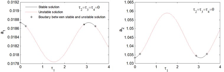
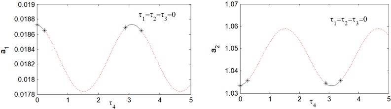
Fig. 5 shows amplitude-delay response curves for . From this figure, we obtain that the amplitude response curves are stable in the delay intervals [0, 0.253] and [2.885, 3.395], otherwise the saturation controlled system becomes unstable. It can be observed from Figs. 2-5 that, for small values of the time delays, the response curve is stable, while when time delays are increased to a critical value, the solution becomes unstable, and this occurs periodically. The interval at which the response curves exhibits stable solution is called vibration reduction region. Fig. 6, show that the response curves of amplitude-delay for increasing excitation forces 0.2, 0.1. It is clear that, when the forcing amplitudes increases the vibration reduction region “solid lines” contracts.
Fig. 3Response amplitude versus time delay τ2
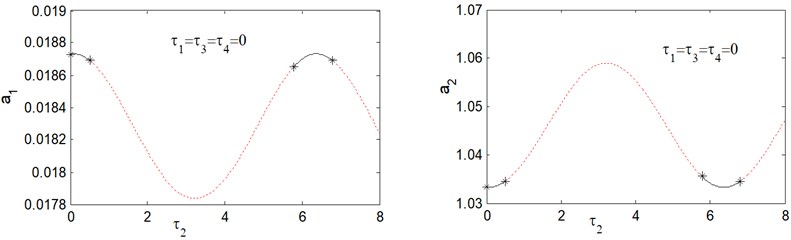
Fig. 4Response amplitude versus time delay τ3
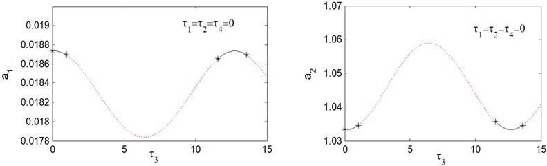
Fig. 5Response amplitude versus time delay τ4
5.2. Frequency response curves of the system without control
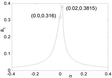
When the amplitude achieves a constant nontrivial value, a steady state vibration exists. Using the frequency response equations, we can determine the influence of the excitation amplitudes, the nonlinear parameter and damping coefficient on the steady state amplitude. The numerical results are shown in Fig. 7, in all figures the region of stability of the nonlinear solutions is determined by applying the Routh-Hurwitz criterion. The solid lines stand for the stable solution and the dotted lines for the unstable solution. From the geometry of the figures, we observe that each curve is continuous and have stable and unstable solution.
Fig. 6Response amplitude versus time delays for increasing excitation forces f1= 0.2, f2= 0.1
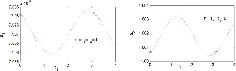
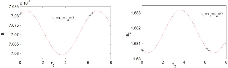
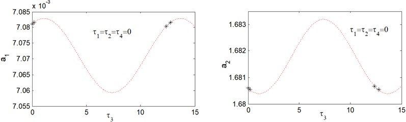
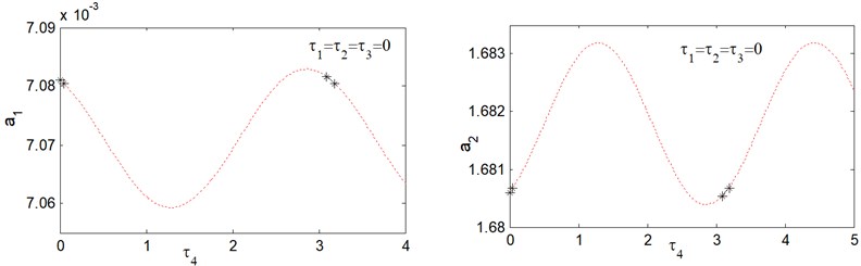
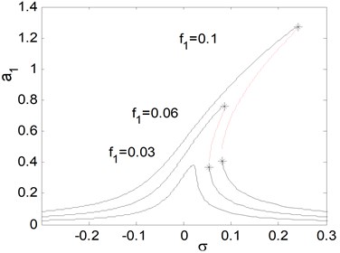
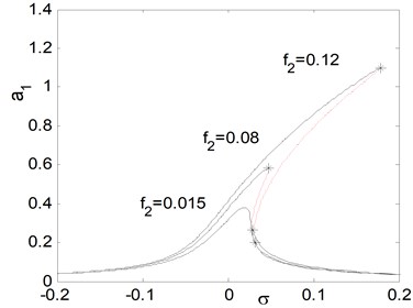
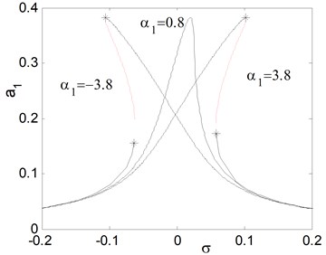
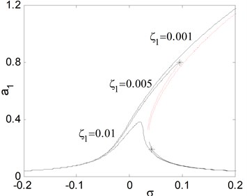
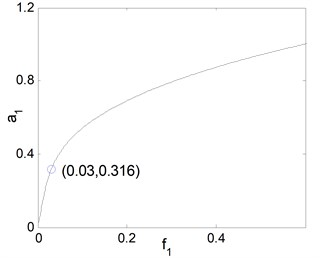
Fig. 7(a), shows the effects of the detuning parameter on the steady state amplitude of the main system when the controller is deactivated. It is clear that from the figure that the maximum steady state amplitude occurs about simultaneous primary and principal parametric resonance when , . Figs. 7(b) and 7(c) shows that the steady state amplitude of the main system is directly proportional to the external and parametric excitation amplitude and respectively. Also, it is clear from Figs. 7(b) and 7(c) that the zone of instability is increased for increasing excitation amplitudes. Fig. 7(d) shows that as the non-linear spring stiffness is increased the continuous curve is moved downwards. Also, the negative and positive values of , produce either hard or soft spring respectively as the curve is either bent to the right or to the left, leading to the appearance of the jump phenomenon. The region of stability is increased for increasing value of . From Fig. 7(e), we observe that the steady state amplitude is inversely proportional to the linear damping coefficient and also for decreasing the curve is bending to the left with increasing region of instability. Fig. 8 represents the external and parametric excitation-response curves for the main system without controller (the controller is deactivated) at simultaneous primary and principal parametric resonance (0) at the same value of the parameters shown in Fig. 7. Fig. 8(a) shows that the response amplitude has a continuous stable curve, which is directly proportional to the excitation amplitude . From Fig. 8(b), we observe that the curve consists of two branches; the upper branch is stable while the down branch has stable and unstable solutions. Also, there exist zone of multi-valued solutions.
Fig. 7Frequency response curves of the main system when the controller is deactivated
a) Effects of the detuning parameter for 0.01, 0.03, 0.015, 0.8, 2
b) Effects of external excitation
c) Effects of parametric excitation
d) Effects of the non-linear parameter
e) Effects of the linear damping
Fig. 8Force response curves of mixed excitation f1 and f2 when the controller is deactivated
a) Force response curves of excitation :
b) Force response curves of excitation 0.01, 0.03, 0.8, 2,0
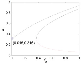
Fig. 9 shows that the external excitation-response curve of the main system and controller (the controller is activated) for time delays 0. Fig. 9 shows that the steady state amplitude is different from Fig. 8(a), since every high steady state amplitude in Fig. 8(a) becomes unstable in Fig. 9. Also, as shown in Fig. 9, as the external excitation force increases the main system’s amplitude saturates and all excess energy due to the external excitation force is channeled to the controller as shown in Fig. 9. That confirms the well-known saturation phenomenon. Fig. 10 shows that the effect of time delays on force-response curves for chosen values are 0.2, 0.3, 0.5, 0.01. Fig. 10 confirm that the saturation phenomenon, but it should be noted that when the time delays increases the stable regions is decreases.
Fig. 9Force response curves of external excitation f1 when the controller is activated for τ1=τ2=τ3=τ4= 0
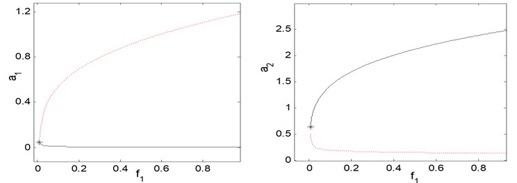
Fig. 10Force response curves of external excitation f1 when the controller is activated for τ1= 0.2, τ2= 0.3, τ3= 0.5, τ4= 0.01
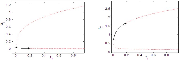
Fig. 11Force response curves of parametric excitation f2 when the controller is activated for τ1=τ2=τ3=τ4= 0
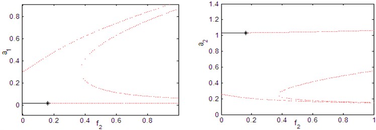
Fig. 12Force response curves of parametric excitation f2 when the controller is activated for τ1= 0.2, τ2=τ3=τ4= 0
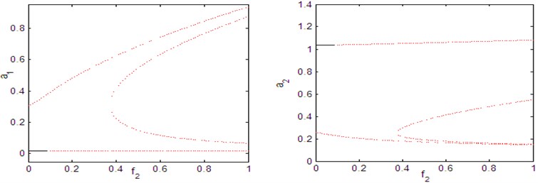
Fig. 11 shows that the parametric excitation-response curve of the main system and controller for time delays 0. Fig. 11 shows that the steady state amplitude is different from Fig. 8(b), since every high steady state amplitude in Fig. 8(b) becomes unstable in Fig. 11. Also, as shown in Fig. 11, as the parametric excitation force increases the main system’s amplitude saturates and all excess energy due to the parametric excitation force is channeled to the controller as shown in Fig. 11. That confirms the well-known saturation phenomenon. Fig. 12 shows that the effect of time delays on force-response curves for chosen values are 0.2, 0, 0, 0. Fig. 12 confirm that the saturation phenomenon, but it should be noted that when the time delays increases the stable regions is decreases.
5.3. Time histories and phase plane
A good criterion of both stability and dynamic chaos is the phase-plane trajectories, which are shown for the considered cases. The various parameters of the plant in Fig. 13 are 0.01, 0.03, 0.015, 0.8, 2, 1, 1, for initial conditions 0, 0. Fig. 13 shows that the steady state amplitude of the plant without controller (controller not in action) at the simultaneous primary and principal parametric resonance is about eleven times the excitation amplitude .
Figs. 14-19 shows that the steady state amplitude of the plant and controller (controller 1:4 internal resonance in action) at simultaneous primary and principle parametric resonance where , in the presence of 1:4 internal resonance for different values of time delays , , , for the same value of the parameters shown in Fig. 2 (i.e. 0.01, 0.001, 0.03, 0.015, 0.8, 2, , 0.2, 0.4) for initial conditions 0, 0.6.
Fig. 13System behavior without controller at resonance Ω1≅ω1, Ω2≅2ω1 for initial conditions u10= 0, u˙1(0)= 0
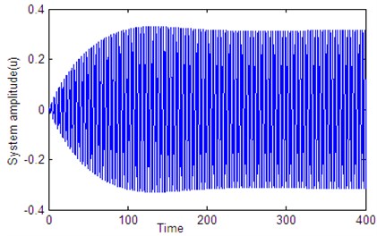
Fig. 14Time histories of the system and controller 1:4 internal resonance when τ1=τ2=τ3=τ4=0, according to initial conditions u1(0)= u˙1(0)=u˙2(0)= 0, u20= 0.6
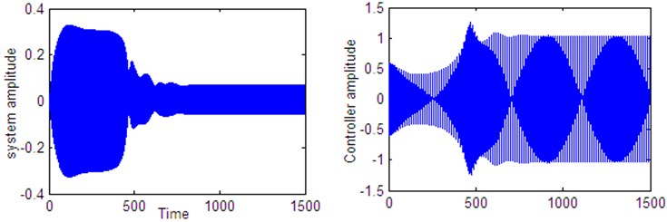
Fig. 15Time histories of the system and controller 1:4 internal resonance when τ1=0.2 according to initial conditions u1(0)= u˙1(0)=u˙2(0)= 0, u20= 0.6
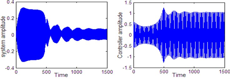
Fig. 16Time histories of the system and controller 1:4 internal resonance when τ1=3.2 according to initial conditions u10= u˙10=u˙20=0, u20= 0.6
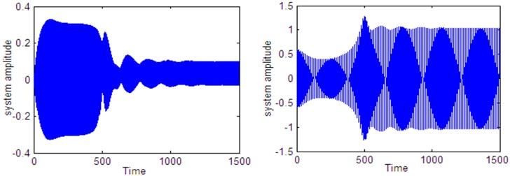
Fig. 17Time histories of the system and controller 1:4 internal resonance when τ3=0.2 according to initial conditions u10= u˙10=u˙20= 0, u20= 0.6
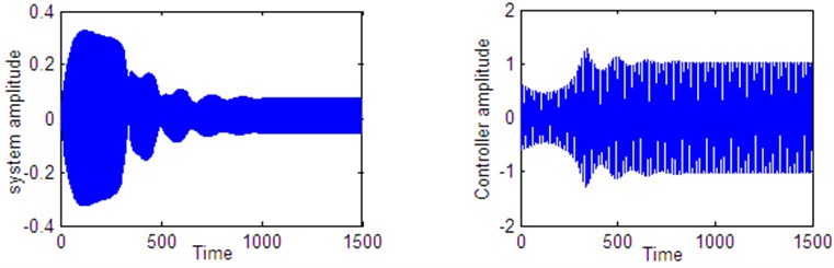
Fig. 18Time histories of the system and controller 1:4 internal resonance when τ4=0.1 according to initial conditions u10= u˙10=u˙20= 0, u20= 0.6
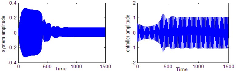
Fig. 19Time histories of the system and controller 1:4 internal resonance when τ3=8 according to initial conditions u1(0)= u˙1(0)=u˙2(0)= 0, u20= 0.6

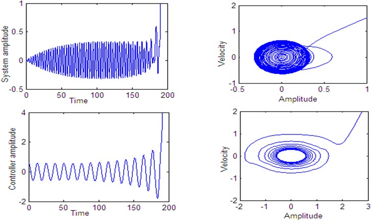
Fig. 14 shows stable behavior for the plant and the controller for 0. From this figure we show that the energy transfers from the main system (plant) to the controller. Figs. 15 to 18, also show stable behavior for the plant and the controller 1:4 internal resonance when the time delay are in the stable region, which taken from Figs. 2 to 5. Fig. 19 shows a complex unstable motion for the plant and the controller when 8 is a way out of the stable range. Figs. 20-23 show unstable behavior for the plant and the controller when one of time delays are in the unstable region.
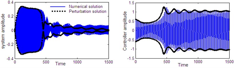
5.4. Numerical validation
To valid the results of multiple time scales perturbation analysis, the set of Eqs. (25)-(28) describes modulation of the amplitudes and the modified phases for the simultaneous primary and principle parametric resonance where in the presence of 1:4 internal resonance . The numerical solutions of Eqs. (25)-(28) for chosen values of system parameters 0.01, 0.001, 0.03, 0.015, 0.8, 2, 0.2, 0.4 at initial conditions 0.6. Figs. 24 and 25 shows that the comparison between numerical integration for the controlled system Eqs. (3)-(4) represented by solid blue lines and the amplitude phase modulating of Eqs. (25)-(28) which obtained from multiple time scales perturbation represented by dashed black lines. We found that, all predictions from analytical solutions are in good agreement with the numerical simulation.
Fig. 20Time histories of the system and controller 1:4 internal resonance when τ1=0.5 according to initial conditions u1(0)= u˙1(0)=u˙2(0)= 0, u20= 0.6
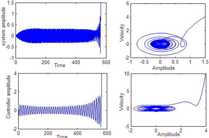
Fig. 21Time histories of the system and controller 1:4 internal resonance when τ2= 2.5 according to initial conditions u1(0)= u˙1(0)=u˙2(0)= 0, u20= 0.6
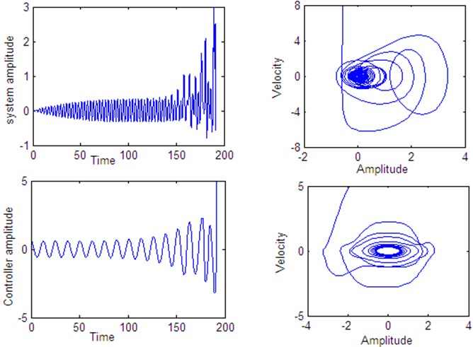
Fig. 22Time histories of the system and controller 1:4 internal resonance when τ3=4 according to initial conditions u1(0)= u˙1(0)=u˙2(0)= 0, u20= 0.6
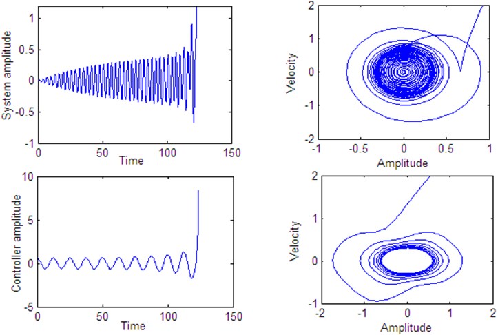
Fig. 23Time histories of the system and controller 1:4 internal resonance when τ4=2 according to initial conditions u1(0)= u˙1(0)=u˙2(0)= 0, u2(0)= 0.6
5.5. Frequency response curves of the controlled system
In the following section, we discuss the effects of the control parameters , , on the behavior of the controlled system.
a) Effects of the control signal .
Figs. 26 and 29 illustrates that for decreasing the control signal on the amplitude response curves against and , we can extend the effective frequency bandwidth of the saturation controller and increase the vibration reduction effect of the main system. Also, we note that the overload risk of the controller decreases as the control signal increases.
Fig. 24Comparison between numerical solution (using RKM) and analytical solution (using perturbation method) of the system and controller 1:4 internal resonance at resonance case when τ1=τ2=τ3=τ4= 0 according to initial conditions u10= u˙10=u˙20= 0, u20= 0.6
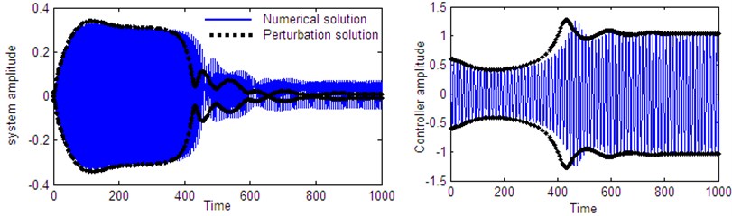
Fig. 25Comparison between numerical solution (using RKM) and analytical solution (using perturbation method) of the system and controller 1:4 internal resonance at resonance case when τ1=0.2 according to initial conditions u1(0)= u˙1(0)=u˙2(0)= 0, u20= 0.6
b) Effects of the feedback signal .
Figs. 27 and 30 illustrates that for increasing the feedback signal on the amplitude response curves against and , we can extend the effective frequency bandwidth of the saturation controller and increase the vibration reduction effect of the main system. Also, we observe that the overload risk of the controller decreases as the feedback signal increases.
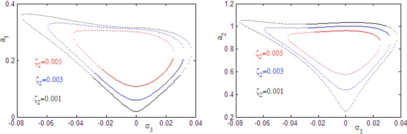
c) Effects of the controller damping coefficient .
Figs. 28 and 31 shows that the effects of the controller damping on the amplitude response curves against and . Form these figure we noticed that for decreasing of the controller damping coefficient the effective frequency bandwidth of the controller and the better of vibration reduction effect of the main system.
Fig. 26Effect of control signal G1 on frequency response of the system a1 and controller a2
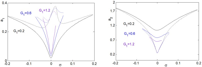
Fig. 27Effect of feedback signal G2 on frequency response of the system a1 and controller a2
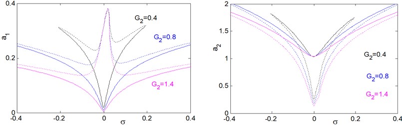
Fig. 28Effect of controller damping coefficient ζ2 on the frequency response of the system a1 and controller a2
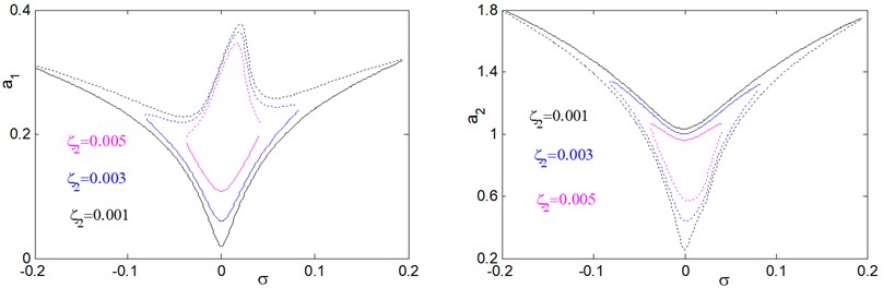
Fig. 29Effect of control signal G1 on the frequency response of the system a1 and controller a2
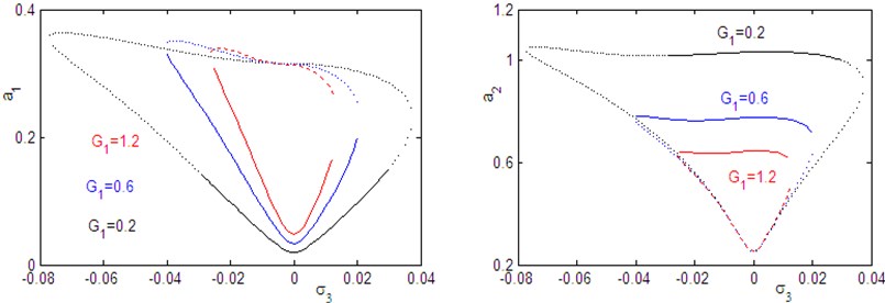
Fig. 30Effect of feedback signal G2 on the frequency response of the system a1 and controller a2
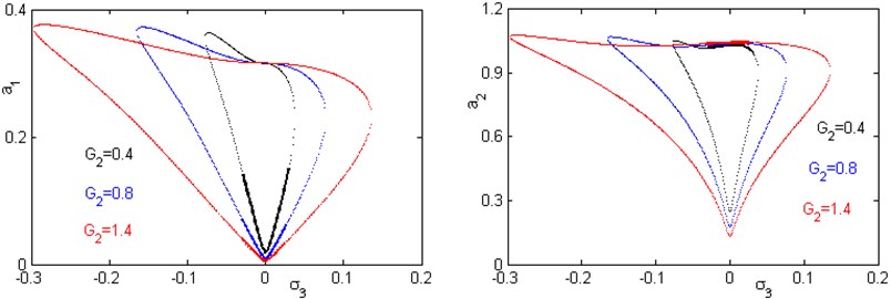
Fig. 31Effect of controller damping coefficient ζ2 on the frequency response of the system a1 and controller a2
6. Conclusions
The nonlinear time delay saturation-controller has been studied for the simultaneous primary and principal parametric resonance in the presence of 1:4 internal resonance. An approximate solution is obtained applying the multiple scales perturbation technique to analyze the nonlinear behavior of the considered system. The stability of the system is investigated applying Lyapunov first method. The frequency response curves are applying to examine the stability of the controlled system and to investigate the performance of the controller. From the above study, the following may be concluded:
1) We can use time delays as a control parameter for suppression the vibration of the system.
2) The interval of the saturation control can be varied by using particular values of time delays.
3) For increasing values of excitation forces, the vibration suppression region is contracts.
4) The analytical solutions are in good agreement with the numerical integrations.
5) Despite of time delays can be applied for stabilizing unstable systems; it also can be used for generating chaotic motions from stable system by applying particular values of time delays.
References
-
Gu K., Kharitonov V. L., Chen J. Stability of Time-Delay Systems. Birkhauser, Boston, MA, 2003.
-
Mazenc F., Niculescu S.-I. Lyapunov stability analysis for nonlinear delay systems. Systems and Control Letters, Vol. 42, Issue 4, 2001, p. 245-251.
-
Niculescu S.-I. Delay Effects on Stability: A Robust Control Approach. Lecture Notes in Control and Information Science, Springer, New York, Berlin, Heidelberg, 2001.
-
Aleksandrov A. Yu., Zhabko A. P. On the stability of the solutions of a class of nonlinear delay systems. Automation and Remote Control, Vol. 67, Issue 9, 2006, p. 1355-1365.
-
Hale Jack K., Verduyn L., Sjoerd M. Introduction to Functional Differential Equations. Springer-Verlag, New York, 1993.
-
Yabuno H., Jo H. Parametric resonance due to asymmetric nonlinearity of restoring force. Journal of System Design and Dynamics, Vol. 2, Issue 3, 2008, p. 898-907.
-
Jo H., Yabuno H. Amplitude reduction of primary resonance of nonlinear oscillator by a dynamic vibration absorber using nonlinear coupling. Nonlinear Dynamics, Vol. 55, Issue 1, 2009, p. 67-78.
-
Jo H., Yabuno H. Amplitude reduction of parametric resonance by dynamic vibration absorber based on quadratic nonlinear coupling. Journal of Sound and Vibration, Vol. 329, Issue 11, 2010, p. 2205-2217.
-
Amer Y. A., Bauomy H. S., Sayed M. Vibration suppression in a twin-tail system to parametric and external excitation. Computers and Mathematics with Applications, Vol. 58, Issue 10, 2009, p. 1947-1964.
-
Hamed Y. S., Sayed M., Cao D.-X., Zhang W. Nonlinear study of the dynamic behavior of a string-beam coupled system under combined excitations. Acta Mechanica Sinica, Vol. 27, Issue 6, 2011, p. 1034-1051.
-
Sayed M., Kamel M. Stability study and control of helicopter blade flapping vibrations. Applied Mathematical Modelling, Vol. 35, Issue 6, 2011, p. 2820-2837.
-
Sayed M., Kamel M. 1:2 and 1:3 internal resonance active absorber for non-linear vibrating system. Applied Mathematical Modelling, Vol. 36, Issue 1, 2012, p. 310-332.
-
Sayed M., Mousa A. A. Second-order approximation of angle-ply composite laminated thin plate under combined excitations. Communication in Nonlinear Science and Numerical Simulation, Vol. 17, Issue 12, 2012, p. 5201-5216.
-
Sayed M., Mousa A. A. Vibration, stability, and resonance of angle-ply composite laminated rectangular thin plate under multi-excitations. Mathematical Problems in Engineering, 2013, p. 418374.
-
Sayed M., Hamed Y. S. Stability analysis and response of nonlinear rotor-seal system. Journal of Vibroengineering, Vol. 16, Issue 8, 2014, p. 4152-4170.
-
Warminski J., Bochenski M., Jarzyna W., Filipek P., Augustyniak M. Active suppression of nonlinear composite beam vibrations by selected control algorithms. Communications in Nonlinear Science and Numerical Simulation, Vol. 16, Issue 5, 2011, p. 2237-2248.
-
Shin C., Hong C., Jeong W. B. Active vibration control of clamped beams using positive position feedback controllers with moment pair. Journal of Mechanical Science and Technology, Vol. 26, Issue 3, 2012, p. 731-740.
-
Eissa M., Sayed M. A comparison between passive and active control of non-linear simple pendulum Part-I. Mathematical and Computational Applications, Vol. 11, Issue 2, 2006, p. 137-149.
-
Eissa M., Sayed M. A comparison between passive and active control of non-linear simple pendulum Part-II. Mathematical and Computational Applications, Vol. 11, Issue 2, 2006, p. 151-162.
-
Eissa M., Sayed M. Vibration reduction of a three DOF non-linear spring pendulum. Communication in Nonlinear Science and Numerical Simulation, Vol. 13, Issue 2, 2008, p. 465–488.
-
Das S. L., Chatterjee A. Multiple scales without center manifold reductions for delay differential equations near Hopf bifurcations. Nonlinear Dynamics, Vol. 30, Issue 4, 2002, p. 323-335.
-
Ahlborn A., Parlitz U. Controlling dynamical systems using multiple delay feedback control. Physical Review E, Vol. 72, 2005, p. 016206.
-
Gjurchinovski A., Jüngling T., Urumov V., Schöll E. Delayed feedback control of unstable steady states with high-frequency modulation of the delay. Physical Review E, Vol. 88, 2013, p. 32912.
-
Zhao Y. Y., Xu J. Effects of delayed feedback control on nonlinear vibration absorber system. Journal of Sound and Vibration, Vol. 308, Issues 1-2, 2007, p. 212-230.
-
Zhao Y. Y., Xu J. Using the delayed feedback control and saturation control to suppress the vibration of dynamical system. Nonlinear Dynamics, Vol. 67, Issue 1, 2012, p. 735-753.
-
Xu J., Chung K. W., Zhao Y. Y. Delayed saturation controller for vibration suppression in stainless-steel beam. Nonlinear Dynamics, Vol. 62, Issue 1, 2010, p. 177-193.
-
Maccari A. Vibration control for the primary resonance of a cantilever beam by a time delay state feedback. Journal of Sound and Vibration, Vol. 259, Issue 2, 2003, p. 241-251.
-
Jnifene A. Active vibration control of flexible structures using delayed position feedback. Systems and Control Letters, Vol. 56, Issue 3, 2007, p. 215-222.
-
Chatterjee S. Time-delay feedback control of friction-induced instability. International Journal of Non-Linear Mechanics, Vol. 42, Issue 9, 2007, p. 1127-1143.
-
Saeed N. A., El-Ganini W. A., Eissa M. Nonlinear time delay saturation-based controller for suppression of nonlinear beam vibrations. Applied Mathematical Modelling, Vol. 37, Issues 20-21, 2013, p. 8846-8864.
-
Song J., He S. Finite-time robust passive control for a class of uncertain Lipschitz nonlinear systems with time-delays. Neurocomputing, Vol. 159, 2015, p. 275-281.
-
Elnaggar A. M., Khalil K. M. The response of nonlinear controlled system under an external excitation via time delay state feedback. Journal of King Saud University – Engineering Sciences, Vol. 28, Issue 1, 2016, p. 75-83.
-
Nayfeh A. H. Introduction to Perturbation Techniques. John Wiley and Sons, Inc., New York, 1981.
-
Nayfeh A. H. Non-linear Interactions. Wiley-Inter-Science, New York, 2000.
-
Nayfeh A. H., Mook D. T. Perturbation Methods. John Wiley and Sons, Inc., 1973.
Cited by
About this article

The authors would like to express their gratitude to the Editor and Referees for their encouragement and constructive comments in revising the paper.
